- Trang chủ >>
- Khoa Học Tự Nhiên >>
- Vật lý
Essential physics 1
Bạn đang xem bản rút gọn của tài liệu. Xem và tải ngay bản đầy đủ của tài liệu tại đây (431.93 KB, 209 trang )
E S S E N T I A L P H Y S I C S
P a r t 1
R E L A T I V I T Y , P A R T I C L E D Y N A M I C S , G R A V I T A T I O N ,
A N D W A V E M O T I O N
F R A N K W . K . F I R K
P r o f e s s o r E m e r i t u s o f P h y s i c s
Y a l e U n i v e r s i t y
2 0 0 0
PREFACE
Throughout the decade of the 1990’s, I taught a one-year course of a specialized nature to
students who entered Yale College with excellent preparation in Mathematics and the
Physical Sciences, and who expressed an interest in Physics or a closely related field. The
level of the course was that typified by the Feynman Lectures on Physics. My one-year
course was necessarily more restricted in content than the two-year Feynman Lectures.
The depth of treatment of each topic was limited by the fact that the course consisted of a
total of fifty-two lectures, each lasting one-and-a-quarter hours. The key role played by
invariants in the Physical Universe was constantly emphasized . The material that I
covered each Fall Semester is presented, almost verbatim, in this book.
The first chapter contains key mathematical ideas, including some invariants of
geometry and algebra, generalized coordinates, and the algebra and geometry of vectors.
The importance of linear operators and their matrix representations is stressed in the early
lectures. These mathematical concepts are required in the presentation of a unified
treatment of both Classical and Special Relativity. Students are encouraged to develop a
“relativistic outlook” at an early stage . The fundamental Lorentz transformation is
developed using arguments based on symmetrizing the classical Galilean transformation.
Key 4-vectors, such as the 4-velocity and 4-momentum, and their invariant norms, are
shown to evolve in a natural way from their classical forms. A basic change in the subject
matter occurs at this point in the book. It is necessary to introduce the Newtonian
concepts of mass, momentum, and energy, and to discuss the conservation laws of linear
and angular momentum, and mechanical energy, and their associated invariants. The
iv
discovery of these laws, and their applications to everyday problems, represents the high
point in the scientific endeavor of the 17th and 18th centuries. An introduction to the
general dynamical methods of Lagrange and Hamilton is delayed until Chapter 9, where
they are included in a discussion of the Calculus of Variations. The key subject of
Einsteinian dynamics is treated at a level not usually met in at the introductory level. The
4-momentum invariant and its uses in relativistic collisions, both elastic and inelastic, is
discussed in detail in Chapter 6. Further developments in the use of relativistic invariants
are given in the discussion of the Mandelstam variables, and their application to the study
of high-energy collisions. Following an overview of Newtonian Gravitation, the general
problem of central orbits is discussed using the powerful method of [p, r] coordinates.
Einstein’s General Theory of Relativity is introduced using the Principle of Equivalence and
the notion of “extended inertial frames” that include those frames in free fall in a
gravitational field of small size in which there is no measurable field gradient. A heuristic
argument is given to deduce the Schwarzschild line element in the “weak field
approximation”; it is used as a basis for a discussion of the refractive index of space-time in
the presence of matter. Einstein’s famous predicted value for the bending of a beam of
light grazing the surface of the Sun is calculated. The Calculus of Variations is an
important topic in Physics and Mathematics; it is introduced in Chapter 9, where it is
shown to lead to the ideas of the Lagrange and Hamilton functions. These functions are
used to illustrate in a general way the conservation laws of momentum and angular
momentum, and the relation of these laws to the homogeneity and isotropy of space. The
subject of chaos is introduced by considering the motion of a damped, driven pendulum.
v
A method for solving the non-linear equation of motion of the pendulum is outlined. Wave
motion is treated from the point-of-view of invariance principles. The form of the general
wave equation is derived, and the Lorentz invariance of the phase of a wave is discussed in
Chapter 12. The final chapter deals with the problem of orthogonal functions in general,
and Fourier series, in particular. At this stage in their training, students are often under-
prepared in the subject of Differential Equations. Some useful methods of solving ordinary
differential equations are therefore given in an appendix.
The students taking my course were generally required to take a parallel one-year
course in the Mathematics Department that covered Vector and Matrix Algebra and
Analysis at a level suitable for potential majors in Mathematics.
Here, I have presented my version of a first-semester course in Physics — a version
that deals with the essentials in a no-frills way. Over the years, I demonstrated that the
contents of this compact book could be successfully taught in one semester. Textbooks
are concerned with taking many known facts and presenting them in clear and concise
ways; my understanding of the facts is largely based on the writings of a relatively small
number of celebrated authors whose work I am pleased to acknowledge in the
bibliography.
Guilford, Connecticut
February, 2000
CONTENTS
1 MATHEMATICAL PRELIMINARIES
1.1 Invariants 1
1.2 Some geometrical invariants 2
1.3 Elements of differential geometry 5
1.4 Gaussian coordinates and the invariant line element 7
1.5 Geometry and groups 10
1.6 Vectors 13
1.7 Quaternions 13
1.8 3-vector analysis 16
1.9 Linear algebra and n-vectors 18
1.10 The geometry of vectors 21
1.11 Linear operators and matrices 24
1.12 Rotation operators 25
1.13 Components of a vector under coordinate rotations 27
2 KINEMATICS: THE GEOMETRY OF MOTION
2.1 Velocity and acceleration 33
2.2 Differential equations of kinematics 36
2.3 Velocity in Cartesian and polar coordinates 39
2.4 Acceleration in Cartesian and polar coordinates 41
3 CLASSICAL AND SPECIAL RELATIVITY
3.1 The Galilean transformation 46
3.2 Einstein’s space-time symmetry: the Lorentz transformation 48
3.3 The invariant interval: contravariant and covariant vectors 51
3.4 The group structure of Lorentz transformations 53
3.5 The rotation group 56
3.6 The relativity of simultaneity: time dilation and length contraction 57
3.7 The 4-velocity 61
4 NEWTONIAN DYNAMICS
4.1 The law of inertia 65
4.2 Newton’s laws of motion 67
4.3 Systems of many interacting particles: conservation of linear and angular
vii
momentum 68
4.4 Work and energy in Newtonian dynamics 74
4.5 Potential energy 76
4.6 Particle interactions 79
4.7 The motion of rigid bodies 84
4.8 Angular velocity and the instantaneous center of rotation 86
4.9 An application of the Newtonian method 88
5 INVARIANCE PRINCIPLES AND CONSERVATION LAWS
5.1 Invariance of the potential under translations and the conservation of linear
momentum 94
5.2 Invariance of the potential under rotations and the conservation of angular
momentum 94
6 EINSTEINIAN DYNAMICS
6.1 4-momentum and the energy-momentum invariant 97
6.2 The relativistic Doppler shift 98
6.3 Relativistic collisions and the conservation of 4- momentum 99
6.4 Relativistic inelastic collisions 102
6.5 The Mandelstam variables 103
6.6 Positron-electron annihilation-in-flight 106
7 NEWTONIAN GRAVITATION
7.1 Properties of motion along curved paths in the plane 111
7.2 An overview of Newtonian gravitation 113
7.3 Gravitation: an example of a central force 118
7.4 Motion under a central force and the conservation of angular momentum 120
7.5 Kepler’s 2nd law explained 120
7.6 Central orbits 121
7.7 Bound and unbound orbits 126
7.8 The concept of the gravitational field 128
7.9 The gravitational potential 131
8 EINSTEINIAN GRAVITATION: AN INTRODUCTION TO GENERAL RELATIVITY
8.1 The principle of equivalence 136
8.2 Time and length changes in a gravitational field 138
8.3 The Schwarzschild line element 138
8.4 The metric in the presence of matter 141
8.5 The weak field approximation 142
viii
8.6 The refractive index of space-time in the presence of mass 143
8.7 The deflection of light grazing the sun 144
9 AN INTRODUCTION TO THE CALCULUS OF VARIATIONS
9.1 The Euler equation 149
9.2 The Lagrange equations 151
9.3 The Hamilton equations 153
10 CONSERVATION LAWS, AGAIN
10.1 The conservation of mechanical energy 158
10.2 The conservation of linear and angular momentum 158
11 CHAOS
11.1 The general motion of a damped, driven pendulum 161
11.2 The numerical solution of differential equations 163
12 WAVE MOTION
12.1 The basic form of a wave 167
12.2 The general wave equation 170
12.3 The Lorentz invariant phase of a wave and the relativistic Doppler shift 171
12.4 Plane harmonic waves 173
12.5 Spherical waves 174
12.6 The superposition of harmonic waves 176
12.7 Standing waves 177
13 ORTHOGONAL FUNCTIONS AND FOURIER SERIES
13.1 Definitions 179
13.2 Some trigonometric identities and their Fourier series 180
13.3 Determination of the Fourier coefficients of a function 182
13.4 The Fourier series of a periodic saw-tooth waveform 183
APPENDIX A SOLVING ORDINARY DIFFERENTIAL EQUATIONS 187
BIBLIOGRAPHY 198
1
MATHEMATICAL PRELIMINARIES
1.1 Invariants
It is a remarkable fact that very few fundamental laws are required to describe the
enormous range of physical phenomena that take place throughout the universe. The
study of these fundamental laws is at the heart of Physics. The laws are found to have a
mathematical structure; the interplay between Physics and Mathematics is therefore
emphasized throughout this book. For example, Galileo found by observation, and
Newton developed within a mathematical framework, the Principle of Relativity:
the laws governing the motions of objects have the same mathematical
form in all inertial frames of reference.
Inertial frames move at constant speed in straight lines with respect to each other – they
are non-accelerating. We say that Newton’s laws of motion are invariant under the
Galilean transformation (see later discussion). The discovery of key invariants of Nature
has been essential for the development of the subject.
Einstein extended the Newtonian Principle of Relativity to include the motions of
beams of light and of objects that move at speeds close to the speed of light. This
extended principle forms the basis of Special Relativity. Later, Einstein generalized the
principle to include accelerating frames of reference. The general principle is known as
the Principle of Covariance; it forms the basis of the General Theory of Relativity ( a theory
of Gravitation).
2 M A T H E M A T I C A L P R E L I M I N A R I E S
A review of the elementary properties of geometrical invariants, generalized
coordinates, linear vector spaces, and matrix operators, is given at a level suitable for a
sound treatment of Classical and Special Relativity. Other mathematical methods,
including contra- and covariant 4-vectors, variational principles, orthogonal functions, and
ordinary differential equations are introduced, as required.
1.2 Some geometrical invariants
In his book The Ascent of Man, Bronowski discusses the lasting importance of the
discoveries of the Greek geometers. He gives a proof of the most famous theorem of
Euclidean Geometry, namely Pythagoras’ theorem, that is based on the invariance of
length and angle ( and therefore of area) under translations and rotations in space. Let a
right-angled triangle with sides a, b, and c, be translated and rotated into the following
four positions to form a square of side c:
c
1
c
2 4
c
b
a 3
c
|← (b – a) →|
The total area of the square = c
2
= area of four triangles + area of shaded square.
If the right-angled triangle is translated and rotated to form the rectangle:
M A T H E M A T I C A L P R E L I M I N A R I E S 3
a a
1 4
b b
2 3
then the area of four triangles = 2ab.
The area of the shaded square area is (b – a)
2
= b
2
– 2ab + a
2
We have postulated the invariance of length and angle under translations and rotations and
therefore
c
2
= 2ab + (b – a)
2
= a
2
+ b
2
. (1.1)
We shall see that this key result characterizes the locally flat space in which we live. It is
the only form that is consistent with the invariance of lengths and angles under
translations and rotations .
The scalar product is an important invariant in Mathematics and Physics. Its invariance
properties can best be seen by developing Pythagoras’ theorem in a three-dimensional
coordinate form. Consider the square of the distance between the points P[x
1
, y
1
, z
1
] and
Q[x
2
, y
2
, z
2
] in Cartesian coordinates:
4 M A T H E M A T I C A L P R E L I M I N A R I E S
z
y
Q[x
2
,y
2
,z
2
]
P[x
1
,y
1
,z
1
]
α
O
x
1
x
2
x
We have
(PQ)
2
= (x
2
– x
1
)
2
+ (y
2
– y
1
)
2
+ (z
2
– z
1
)
2
= x
2
2
– 2x
1
x
2
+ x
1
2
+ y
2
2
– 2y
1
y
2
+ y
1
2
+ z
2
2
– 2z
1
z
2
+ z
1
2
= (x
1
2
+ y
1
2
+ z
1
2
) + (x
2
2
+ y
2
2
+ z
2
2
) – 2(x
1
x
2
+ y
1
y
2
+ z
1
z
2
)
= (OP)
2
+ (OQ)
2
– 2(x
1
x
2
+ y
1
y
2
+ z
1
z
2
) (1.2)
The lengths PQ, OP, OQ, and their squares, are invariants under rotations and therefore
the entire right-hand side of this equation is an invariant. The admixture of the
coordinates (x
1
x
2
+ y
1
y
2
+ z
1
z
2
) is therefore an invariant under rotations. This term has a
geometric interpretation: in the triangle OPQ, we have the generalized Pythagorean
theorem
(PQ)
2
= (OP)
2
+ (OQ)
2
– 2OP.OQ cosα,
therefore
OP.OQ cosα = x
1
x
2
+y
1
y
2
+ z
1
z
2
≡ the scalar product. (1.3)
Invariants in space-time with scalar-product-like forms, such as the interval
between events (see 3.3), are of fundamental importance in the Theory of Relativity.
M A T H E M A T I C A L P R E L I M I N A R I E S 5
Although rotations in space are part of our everyday experience, the idea of rotations in
space-time is counter-intuitive. In Chapter 3, this idea is discussed in terms of the relative
motion of inertial observers.
1.3 Elements of differential geometry
Nature does not prescibe a particular coordinate system or mesh. We are free to
select the system that is most appropriate for the problem at hand. In the familiar
Cartesian system in which the mesh lines are orthogonal, equidistant, straight lines in the
plane, the key advantage stems from our ability to calculate distances given the
coordinates – we can apply Pythagoras’ theorem, directly. Consider an arbitrary mesh:
v – direction P[3
u
, 4
v
]
4
v
ds, a length
3
v
dv
α
du
2
v
1
v
Origin O 1
u
2
u
3
u
u – direction
Given the point P[3
u
, 4
v
], we cannot use Pythagoras’ theorem to calculate the distance
OP.
6 M A T H E M A T I C A L P R E L I M I N A R I E S
In the infinitesimal parallelogram shown, we might think it appropriate to write
ds
2
= du
2
+ dv
2
+ 2dudvcosα . (ds
2
= (ds)
2
, a squared “length” )
This we cannot do! The differentials du and dv are not lengths – they are simply
differences between two numbers that label the mesh. We must therefore multiply each
differential by a quantity that converts each one into a length. Introducing dimensioned
coefficients, we have
ds
2
= g
11
du
2
+ 2g
12
dudv + g
22
dv
2
(1.4)
where √g
11
du and √g
22
dv are now lengths.
The problem is therefore one of finding general expressions for the coefficients;
it was solved by Gauss, the pre-eminent mathematician of his age. We shall restrict our
discussion to the case of two variables. Before treating this problem, it will be useful to
recall the idea of a total differential associated with a function of more than one variable.
Let u = f(x, y) be a function of two variables, x and y. As x and y vary, the corresponding
values of u describe a surface. For example, if u = x
2
+ y
2
, the surface is a paraboloid of
revolution. The partial derivatives of u are defined by
∂f(x, y)/∂x = limit as h →0 {(f(x + h, y) – f(x, y))/h} (treat y as a constant), (1.5)
and
∂f(x, y)/∂y = limit as k →0 {(f(x, y + k) – f(x, y))/k} (treat x as a constant). (1.6)
For example, if u = f(x, y) = 3x
2
+ 2y
3
then
∂f/∂x = 6x, ∂
2
f/∂x
2
= 6, ∂
3
f/∂x
3
= 0
and
M A T H E M A T I C A L P R E L I M I N A R I E S 7
∂f/∂y = 6y
2
, ∂
2
f/∂y
2
= 12y, ∂
3
f/∂y
3
= 12, and ∂
4
f/∂y
4
= 0.
If u = f(x, y) then the total differential of the function is
du = (∂f/∂x)dx + (∂f/∂y)dy
corresponding to the changes: x → x + dx and y → y + dy.
(Note that du is a function of x, y, dx, and dy of the independent variables x and y)
1.4 Gaussian coordinates and the invariant line element
Consider the infinitesimal separation between two points P and Q that are
described in either Cartesian or Gaussian coordinates:
y + dy Q v + dv Q
ds ds
y P v P
x x + dx u u + du
Cartesian Gaussian
In the Gaussian system, du and dv do not represent distances.
Let
x = f(u, v) and y = F(u, v) (1.7 a,b)
then, in the infinitesimal limit
dx = (∂x/∂u)du + (∂x/∂v)dv and dy = (∂y/∂u)du + (∂y/∂v)dv.
In the Cartesian system, there is a direct correspondence between the mesh-numbers and
distances so that
8 M A T H E M A T I C A L P R E L I M I N A R I E S
ds
2
= dx
2
+ dy
2
. (1.8)
But
dx
2
= (∂x/∂u)
2
du
2
+ 2(∂x/∂u)(∂x/∂v)dudv + (∂x/∂v)
2
dv
2
and
dy
2
= (∂y/∂u)
2
du
2
+ 2(∂y/∂u)(∂y/∂v)dudv + (∂y/∂v)
2
dv
2
.
We therefore obtain
ds
2
= {(∂x/∂u)
2
+ (∂y/∂u)
2
}du
2
+ 2{(∂x/∂u)(∂x/∂v) + (∂y/∂u)(∂y/∂v)}dudv
+ {(∂x/∂v)
2
+ (∂y/∂v)
2
}dv
2
= g
11
du
2
+ 2g
12
dudv + g
22
dv
2
. (1.9)
If we put u = u
1
and v = u
2
, then
ds
2
= ∑ ∑ g
ij
du
i
du
j
where i,j = 1,2. (1.10)
i
j
(This is a general form for an n-dimensional space: i, j = 1, 2, 3, n).
Two important points connected with this invariant differential line element are:
1. Interpretation of the coefficients g
ij
.
Consider a Euclidean mesh of equispaced parallelograms:
v
R
ds
α dv
u
P du Q
M A T H E M A T I C A L P R E L I M I N A R I E S 9
In PQR
ds
2
= 1.du
2
+ 1.dv
2
+ 2cosαdudv
= g
11
du
2
+ g
22
dv
2
+ 2g
12
dudv (1.11)
therefore, g
11
= g
22
= 1 (the mesh-lines are equispaced)
and
g
12
= cosα where α is the angle between the u-v axes.
We see that if the mesh-lines are locally orthogonal then g
12
= 0.
2. Dependence of the g
ij
’s on the coordinate system and the local values of u, v.
A specific example will illustrate the main points of this topic: consider a point P
described in three coordinate systems – Cartesian P[x, y], Polar P[r, φ], and Gaussian
P[u, v] – and the square ds
2
of the line element in each system.
The transformation [x, y] → [r, φ] is
x = rcosφ and y = rsinφ. (1.12 a,b)
The transformation [r, φ] → [u, v] is direct, namely
r = u and φ = v.
Now,
∂x/∂r = cosφ, ∂y/∂r = sinφ, ∂x/∂φ = – rsinφ, ∂y/∂φ = rcosφ
therefore,
∂x/∂u = cosv, ∂y/∂u = sinv, ∂x/∂v = – usinv, ∂y/∂v = ucosv.
The coefficients are therefore
g
11
= cos
2
v + sin
2
v = 1, (1.13 a-c)
1 0 M A T H E M A T I C A L P R E L I M I N A R I E S
g
22
= (–usinv)
2
+(ucosv)
2
= u
2
,
and
g
12
= cos(–usinv) + sinv(ucosv) = 0 (an orthogonal mesh).
We therefore have
ds
2
= dx
2
+ dy
2
(1.14 a-c)
= du
2
+ u
2
dv
2
= dr
2
+ r
2
dφ
2
.
In this example, the coefficient g
22
= f(u).
The essential point of Gaussian coordinate systems is that the coefficients, g
ij
,
completely characterize the surface – they are intrinsic features. We can, in principle,
determine the nature of a surface by measuring the local values of the coefficients as we
move over the surface. We do not need to leave a surface to study its form.
1.5 Geometry and groups
Felix Klein (1849 – 1925), introduced his influential Erlanger Program in 1872. In
this program, Geometry is developed from the viewpoint of the invariants associated with
groups of transformations. In Euclidean Geometry, the fundamental objects are taken to
be rigid bodies that remain fixed in size and shape as they are moved from place to place.
The notion of a rigid body is an idealization.
Klein considered transformations of the entire plane – mappings of the set of all
points in the plane onto itself. The proper set of rigid motions in the plane consists of
translations and rotations. A reflection is an improper rigid motion in the plane; it is a
physical impossibility in the plane itself. The set of all rigid motions – both proper and
M A T H E M A T I C A L P R E L I M I N A R I E S 1 1
improper – forms a group that has the proper rigid motions as a subgroup. A group G is a
set of distinct elements {g
i
} for which a law of composition “
o
” is given such that the
composition of any two elements of the set satisfies:
Closure: if g
i
, g
j
belong to G then g
k
= g
i
o
g
j
belongs to G for all elements g
i
, g
j
,
and
Associativity: for all g
i
, g
j
, g
k
in G, g
i
o
(g
j
o
g
k
) = (g
i
o
g
j
)
o
g
k
. .
Furthermore, the set contains
A unique identity, e, such that g
i
o
e = e
o
g
i
= g
i
for all g
i
in G,
and
A unique inverse, g
i
–1
, for every element g
i
in G,
such that g
i
o
g
i
–1
= g
i
–1
o
g
i
= e.
A group that contains a finite number n of distinct elements g
n
is said to be a finite group
of order n.
The set of integers Z is a subset of the reals R; both sets form infinite groups under
the composition of addition. Z is a “subgroup“of R.
Permutations of a set X form a group S
x
under composition of functions; if a: X → X
and b: X → X are permutations, the composite function ab: X → X given by ab(x) =
a(b(x)) is a permutation. If the set X contains the first n positive numbers, the n!
permutations form a group, the symmetric group, S
n
. For example, the arrangements of
the three numbers 123 form the group
S
3
= { 123, 312, 231, 132, 321, 213 }.
1 2 M A T H E M A T I C A L P R E L I M I N A R I E S
If the vertices of an equilateral triangle are labelled 123, the six possible symmetry
arrangements of the triangle are obtained by three successive rotations through 120
o
about its center of gravity, and by the three reflections in the planes I, II, III:
I
1
2 3
II III
This group of “isometries“of the equilateral triangle (called the dihedral group, D
3
) has the
same structure as the group of permutations of three objects. The groups S
3
and D
3
are
said to be isomorphic.
According to Klein, plane Euclidean Geometry is the study of those properties of
plane rigid figures that are unchanged by the group of isometries. (The basic invariants are
length and angle). In his development of the subject, Klein considered Similarity
Geometry that involves isometries with a change of scale, (the basic invariant is angle),
Affine Geometry, in which figures can be distorted under transformations of the form
x´ = ax + by + c (1.15 a,b)
y´ = dx + ey + f ,
where [x, y] are Cartesian coordinates, and a, b, c, d, e, f, are real coefficients, and
Projective Geometry, in which all conic sections are equivalent; circles, ellipses, parabolas,
and hyperbolas can be transformed into one another by a projective transformation.
M A T H E M A T I C A L P R E L I M I N A R I E S 1 3
It will be shown that the Lorentz transformations – the fundamental transformations of
events in space and time, as described by different inertial observers – form a group.
1.6 Vectors
The idea that a line with a definite length and a definite direction — a vector — can
be used to represent a physical quantity that possesses magnitude and direction is an
ancient one. The combined action of two vectors A and B is obtained by means of the
parallelogram law, illustrated in the following diagram
A + B
B
A
The diagonal of the parallelogram formed by A and B gives the magnitude and direction of
the resultant vector C. Symbollically, we write
C = A + B (1.16)
in which the “=” sign has a meaning that is clearly different from its meaning in ordinary
arithmetic. Galileo used this empirically-based law to obtain the resultant force acting on
a body. Although a geometric approach to the study of vectors has an intuitive appeal, it
will often be advantageous to use the algebraic method – particularly in the study of
Einstein’s Special Relativity and Maxwell’s Electromagnetism.
1.7 Quaternions
In the decade 1830 - 1840, the renowned Hamilton introduced new kinds of
1 4 M A T H E M A T I C A L P R E L I M I N A R I E S
numbers that contain four components, and that do not obey the commutative property of
multiplication. He called the new numbers quaternions. A quaternion has the form
u + xi + yj + zk (1.17)
in which the quantities i, j, k are akin to the quantity i = √–1 in complex numbers,
x + iy. The component u forms the scalar part, and the three components xi + yj + zk
form the vector part of the quaternion. The coefficients x, y, z can be considered to be
the Cartesian components of a point P in space. The quantities i, j, k are qualitative units
that are directed along the coordinate axes. Two quaternions are equal if their scalar parts
are equal, and if their coefficients x, y, z of i, j, k are respectively equal. The sum of two
quaternions is a quaternion. In operations that involve quaternions, the usual rules of
multiplication hold except in those terms in which products of i, j, k occur — in these
terms, the commutative law does not hold. For example
j k = i, k j = – i, k i = j, i k = – j, i j = k, j i = – k, (1.18)
(these products obey a right-hand rule),
and
i
2
= j
2
= k
2
= –1. (Note the relation to i
2
= –1). (1.19)
The product of two quaternions does not commute. For example, if
p = 1 + 2i + 3j + 4k, and q = 2 + 3i + 4j + 5k
then
pq = – 36 + 6i + 12j + 12k
whereas
M A T H E M A T I C A L P R E L I M I N A R I E S 1 5
qp = – 36 + 23i – 2j + 9k.
Multiplication is associative.
Quaternions can be used as operators to rotate and scale a given vector into a new
vector:
(a + bi + cj + dk)(xi + yj + zk) = (x´i + y´j + z´k)
If the law of composition is quaternionic multiplication then the set
Q = {±1, ±i, ±j, ±k}
is found to be a group of order 8. It is a non-commutative group.
Hamilton developed the Calculus of Quaternions. He considered, for example, the
properties of the differential operator:
∇ = i(∂/∂x) + j(∂/∂y) + k(∂/∂z). (1.20)
(He called this operator “nabla”).
If f(x, y, z) is a scalar point function (single-valued) then
∇f = i(∂f/∂x) + j(∂f/∂y) + k(∂f/∂z) , a vector.
If
v = v
1
i + v
2
j + v
3
k
is a continuous vector point function, where the v
i
’s are functions of x, y, and z, Hamilton
introduced the operation
∇v = (i∂/∂x + j∂/∂y + k∂/∂z)(v
1
i + v
2
j + v
3
k) (1.21)
= – (∂v
1
/∂x + ∂v
2
/∂y + ∂v
3
/∂z)
+ (∂v
3
/∂y – ∂v
2
/∂z)i + (∂v
1
/∂z – ∂v
3
/∂x)j + (∂v
2
/∂x – ∂v
1
/∂y)k
1 6 M A T H E M A T I C A L P R E L I M I N A R I E S
= a quaternion.
The scalar part is the negative of the “divergence of v” (a term due to Clifford), and the
vector part is the “curl of v” (a term due to Maxwell). Maxwell used the repeated operator
∇
2
, which he called the Laplacian.
1.8 3 – vector analysis
Gibbs, in his notes for Yale students, written in the period 1881 - 1884, and Heaviside, in
articles published in the Electrician in the 1880’s, independently developed 3-dimensional
Vector Analysis as a subject in its own right — detached from quaternions.
In the Sciences, and in parts of Mathematics (most notably in Analytical and Differential
Geometry), their methods are widely used. Two kinds of vector multiplication were
introduced: scalar multiplication and vector multiplication. Consider two vectors v and v´
where
v = v
1
e
1
+ v
2
e
2
+ v
3
e
3
and
v´ = v
1
´e
1
+ v
2
´e
2
+ v
3
´e
3
.
The quantities e
1
, e
2
, and e
3
are vectors of unit length pointing along mutually orthogonal
axes, labelled 1, 2, and 3.
i) The scalar multiplication of v and v´ is defined as
v ⋅ v´ = v
1
v
1
´ + v
2
v
2
´ + v
3
v
3
´, (1.22)
where the unit vectors have the properties
e
1
⋅ e
1
= e
2
⋅ e
2
= e
3
⋅ e
3
= 1, (1.23)
M A T H E M A T I C A L P R E L I M I N A R I E S 1 7
and
e
1
⋅ e
2
= e
2
⋅ e
1
= e
1
⋅ e
3
= e
3
⋅ e
1
= e
2
⋅ e
3
= e
3
⋅ e
2
= 0. (1.24)
The most important property of the scalar product of two vectors is its invariance
under rotations and translations of the coordinates. (See Chapter 1).
ii) The vector product of two vectors v and v´ is defined as
e
1
e
2
e
3
v × v´ = v
1
v
2
v
3
( where |. . . |is the determinant) (1.25)
v
1
´ v
2
´ v
3
´
= (v
2
v
3
´ – v
3
v
2
´)e
1
+ (v
3
v
1
´ – v
1
v
3
´)e
2
+ (v
1
v
2
´ – v
2
v
1
´)e
3
.
The unit vectors have the properties
e
1
× e
1
= e
2
× e
2
= e
3
× e
3
= 0 (1.26 a,b)
(note that these properties differ from the quaternionic products of the i, j, k’s),
and
e
1
× e
2
= e
3
, e
2
× e
1
= – e
3
, e
2
× e
3
= e
1
, e
3
× e
2
= – e
1
, e
3
× e
1
= e
2
, e
1
× e
3
= – e
2
These non-commuting vectors, or “cross products” obey the standard right-hand-rule.
The vector product of two parallel vectors is zero even when neither vector is zero.
The non-associative property of a vector product is illustrated in the following
example
e
1
× e
2
× e
2
= (e
1
× e
2
) × e
2
= e
3
× e
2
= – e
1
= e
1
× (e
2
× e
2
) = 0.