- Trang chủ >>
- Khoa Học Tự Nhiên >>
- Vật lý
Basics of radio astronomy for the goldstone apple valley radio telescope
Bạn đang xem bản rút gọn của tài liệu. Xem và tải ngay bản đầy đủ của tài liệu tại đây (1.14 MB, 109 trang )
Basics of Radio AstronomyBasics of Radio Astronomy
Basics of Radio AstronomyBasics of Radio Astronomy
Basics of Radio Astronomy
for thefor the
for thefor the
for the
Goldstone-Apple ValleyGoldstone-Apple Valley
Goldstone-Apple ValleyGoldstone-Apple Valley
Goldstone-Apple Valley
Radio TelescopeRadio Telescope
Radio TelescopeRadio Telescope
Radio Telescope
April 1998April 1998
April 1998April 1998
April 1998
JPL D-13835
Basics of Radio AstronomyBasics of Radio Astronomy
Basics of Radio AstronomyBasics of Radio Astronomy
Basics of Radio Astronomy
for thefor the
for thefor the
for the
Goldstone-Apple ValleyGoldstone-Apple Valley
Goldstone-Apple ValleyGoldstone-Apple Valley
Goldstone-Apple Valley
Radio TelescopeRadio Telescope
Radio TelescopeRadio Telescope
Radio Telescope
Prepared byPrepared by
Prepared byPrepared by
Prepared by
Diane Fisher MillerDiane Fisher Miller
Diane Fisher MillerDiane Fisher Miller
Diane Fisher Miller
Advanced Mission Operations SectionAdvanced Mission Operations Section
Advanced Mission Operations SectionAdvanced Mission Operations Section
Advanced Mission Operations Section
Also available on the Internet at URL
/>April 1998April 1998
April 1998April 1998
April 1998
JPL D-13835JPL D-13835
JPL D-13835JPL D-13835
JPL D-13835
JPL D-13835
ii
Document Log
Basics of Radio Astronomy Learner’s Workbook
Document Identifier Date Description
D-13835, Preliminary 3/3/97 Preliminary “Beta” release of document.
D-13835, Final 4/17/98 Final release of document. Adds discussions of
superposition, interference, and diffraction in
Chapter 4.
Copyright ©1997, 1998, California Institute of Technology, Pasadena, California. ALL RIGHTS
RESERVED. Based on Government-sponsored Research NAS7-1260.
BASICS OF RADIO ASTRONOMY
iii
Preface
In a collaborative effort, the Science and Technology Center (in Apple Valley, California), the
Apple Valley Unified School District, the Jet Propulsion Laboratory, and NASA have converted a
34-meter antenna at NASA's Deep Space Network's Goldstone Complex into a unique interactive
research and teaching instrument available to classrooms throughout the United States, via the
Internet. The Science and Technology Center is a branch of the Lewis Center for Educational
Research.
The Goldstone-Apple Valley Radio Telescope (GAVRT) is located in a remote area of the
Mojave Desert, 40 miles north of Barstow, California. The antenna, identified as DSS-12, is a 34-
meter diameter dish, 11 times the diameter of a ten-foot microwave dish used for satellite televi-
sion reception. DSS-12 has been used by NASA to communicate with robotic space probes for
more than thirty years. In 1994, when NASA decided to decommission DSS-12 from its opera-
tional network, a group of professional scientists, educators, engineers, and several community
volunteers envisioned a use for this antenna and began work on what has become the GAVRT
Project.
The GAVRT Project is jointly managed by the Science and Technology Center and the DSN
Science Office, Telecommunications and Mission Operations Directorate, at the Jet Propulsion
Laboratory.
This workbook was developed as part of the training of teachers and volunteers who will be
operating the telescope. The students plan observations and operate the telescope from the Apple
Valley location using Sun workstations. In addition, students and teachers in potentially 10,000
classrooms across the country will be able to register with the center’s Web site and operate the
telescope from their own classrooms.
JPL D-13835
iv
BASICS OF RADIO ASTRONOMY
v
Contents
Introduction 1
Assumptions 1
Disclaimers 1
Learning Strategy 1
Help with Abbreviations and Units of Measure 2
1. Overview: Discovering an Invisible Universe 3
Jansky’s Experiment 3
Reber’s Prototype Radio Telescope 5
So What’s a Radio Telescope? 5
What’s the GAVRT? 6
2. The Properties of Electromagnetic Radiation 9
What is Electromagnetic Radiation? 9
Frequency and Wavelength 9
Inverse-Square Law of Propagation 11
The Electromagnetic Spectrum 12
Wave Polarization 15
3. The Mechanisms of Electromagnetic Emissions 19
Thermal Radiation 19
Blackbody Characteristics 20
Continuum Emissions from Ionized Gas 23
Spectral Line Emission from Atoms and Molecules 23
Non-thermal Mechanisms 26
Synchrotron Radiation 26
Masers 27
4. Effects of Media 29
Atmospheric “Windows” 29
Absorption and Emission Lines 30
Reflection 34
Refraction 35
Superposition 36
Phase 37
Interference 37
Diffraction 38
Scintillation 40
Faraday Rotation 41
5. Effects of Motion and Gravity 43
Doppler Effect 43
Gravitational Red Shifting 44
JPL D-13835
vi
Gravitational Lensing 45
Superluminal Velocities 45
Occultations 47
6. Sources of Radio Frequency Emissions 49
Classifying the Source 49
Star Sources 51
Variable Stars 51
Pulsars 52
Our Sun 54
Galactic and Extragalactic Sources 56
Quasars 57
Planetary Sources and Their Satellites 58
The Jupiter System 58
Sources of Interference 60
7. Mapping the Sky 63
Earth’s Coordinate System 63
Revolution of Earth 64
Solar vs. Sidereal Day 64
Precession of the Earth Axis 66
Astronomical Coordinate Systems 66
Horizon Coordinate System 66
Equatorial Coordinate System 68
Ecliptic Coordinate System 71
Galactic Coordinate System 71
8. Our Place in the Universe 75
The Universe in Six Steps 75
The Search for Extraterrestrial Intelligence 79
Appendix:
A. Glossary 81
B. References and Further Reading 89
Books 89
World Wide Web Sites 90
Video 90
Illustration Credits 91
Index 93
BASICS OF RADIO ASTRONOMY
1
Introduction
This module is the first in a sequence to prepare volunteers and teachers at the Science and
Technology Center to operate the Goldstone-Apple Valley Radio Telescope (GAVRT). It covers
the basic science concepts that will not only be used in operating the telescope, but that will make
the experience meaningful and provide a foundation for interpreting results.
Acknowledgements
Many people contributed to this workbook. The first problem we faced was to decide which of
the overwhelming number of astronomy topics we should cover and at what depth in order to
prepare GAVRT operators for the radio astronomy projects they would likely be performing.
George Stephan generated this initial list of topics, giving us a concrete foundation on which to
begin to build. Thanks to the subject matter experts in radio astronomy, general astronomy, and
physics who patiently reviewed the first several drafts and took time to explain some complex
subjects in plain English for use in this workbook. These kind reviewers are Dr. M.J. Mahoney,
Roger Linfield, David Doody, Robert Troy, and Dr. Kevin Miller (who also loaned the project
several most valuable books from his personal library). Special credit goes to Dr. Steve Levin,
who took responsibility for making sure the topics covered were the right ones and that no known
inaccuracies or ambiguities remained. Other reviewers who contributed suggestions for clarity
and completeness were Ben Toyoshima, Steve Licata, Kevin Williams, and George Stephan.
Assumptions and Disclaimers
This training module assumes you have an understanding of high-school-level chemistry, physics,
and algebra. It also assumes you have familiarity with or access to other materials on general
astronomy concepts, since the focus here is on those aspects of astronomy that relate most
specifically to radio astronomy.
This workbook does not purport to cover its selected topics in depth, but simply to introduce them
and provide some context within the overall disciplines of astronomy in general and radio as-
tronomy in particular. It does not cover radio telescope technology, nor details of radio as-
tronomy data analysis.
Learning Strategy
As a participant, you study this workbook by yourself. It includes both learning materials and
evaluation tools. The chapters are designed to be studied in the order presented, since some
concepts developed in later chapters depend on concepts introduced in earlier ones. It doesn't
matter how long it takes you to complete it. What is important is that you accomplish all the
learning objectives.
Introduction
JPL D-13835
2
The frequent “Recap” (for recapitulation) sections at the end of each short module will help you
reinforce key points and evaluate your progress. They require you to fill in blanks. Please do so
either mentally or jot your answers on paper. Answers from the text are shown at the bottom of
each Recap. In addition, “For Further Study” boxes appear throughout this workbook suggesting
references that expand on many of the topics introduced. See “References and Further Reading”
on Page 85 for complete citations of these sources.
After you complete the workbook, you will be asked to complete a self-administered quiz (fill in
the blanks) covering all the objectives of the learning module and then send it to the GAVRT
Training Engineer. It is okay to refer to the workbook in completing the final quiz. A score of at
least 90% is expected to indicate readiness for the next module in the GAVRT operations readi-
ness training sequence.
Help with Abbreviations and Units of Measure
This workbook uses standard abbreviations for units of measure. Units of measure are listed
below. Refer to the Glossary in Appendix A for further help. As is the case when you are study-
ing any subject, you should also have a good English dictionary at hand.
k (with a unit of measure) kilo (10
3
, or thousand)
M (with a unit of measure) Mega (10
6
, or million)
G (with a unit of measure) Giga (10
9
, or billion; in countries using the metric
system outside the USA, a billion is 10
12
. Giga, however, is always 10
9
.)
T (with a unit of measure) Tera (10
12
, or a million million)
P (with a unit of measure) Peta (10
15
)
E (with a unit of measure) Exa (10
18
)
Hz Hertz
K Kelvin
m meter (USA spelling; elsewhere, metre)
nm nanometer (10
-9
meter)
BASICS OF RADIO ASTRONOMY
3
Chapter 1
Overview: Discovering an Invisible Universe
Objectives: Upon completion of this chapter, you will be able to describe the general prin-
ciples upon which radio telescopes work.
Before 1931, to study astronomy meant to study the objects visible in the night sky. Indeed, most
people probably still think that’s what astronomers do—wait until dark and look at the sky using
their naked eyes, binoculars, and optical telescopes, small and large. Before 1931, we had no
idea that there was any other way to observe the universe beyond our atmosphere.
In 1931, we did know about the electromagnetic spectrum. We knew that visible light included
only a small range of wavelengths and frequencies of energy. We knew about wavelengths
shorter than visible light—Wilhelm Röntgen had built a machine that produced x-rays in 1895.
We knew of a range of wavelengths longer than visible light (infrared), which in some circum-
stances is felt as heat. We even knew about radio frequency (RF) radiation, and had been devel-
oping radio, television, and telephone technology since Heinrich Hertz first produced radio waves
of a few centimeters long in 1888. But, in 1931, no one knew that RF radiation is also emitted by
billions of extraterrestrial sources, nor that some of these frequencies pass through Earth’s
atmosphere right into our domain on the ground.
All we needed to detect this radiation was a new kind of “eyes.”
Jansky’s Experiment
As often happens in science, RF radiation from outer space was first discovered while someone
was looking for something else. Karl G. Jansky (1905-1950) worked as a radio engineer at the
Bell Telephone Laboratories in Holmdel, New Jersey. In 1931, he was assigned to study radio
frequency interference from thunderstorms in order to help Bell design an antenna that would
minimize static when beaming radio-telephone signals across the ocean. He built an awkward
looking contraption that looked more like a wooden merry-go-round than like any modern-day
antenna, much less a radio telescope. It was tuned to respond to radiation at a wavelength of 14.6
meters and rotated in a complete circle on old Ford tires every 20 minutes. The antenna was
connected to a receiver and the antenna’s output was recorded on a strip-chart recorder.
Overview: Discovering an Invisible Universe
JPL D-13835
4
Jansky’s Antenna that First Detected Extraterrestrial RF Radiation
He was able to attribute some of the static (a term used by radio engineers for noise produced by
unmodulated RF radiation) to thunderstorms nearby and some of it to thunderstorms farther away,
but some of it he couldn’t place. He called it “ . . . a steady hiss type static of unknown origin.”
As his antenna rotated, he found that the direction from which this unknown static originated
changed gradually, going through almost a complete circle in 24 hours. No astronomer himself, it
took him a while to surmise that the static must be of extraterrestrial origin, since it seemed to be
correlated with the rotation of Earth.
He at first thought the source was the sun. However, he observed that the radiation peaked about
4 minutes earlier each day. He knew that Earth, in one complete orbit around the sun, necessarily
makes one more revolution on its axis with respect to the sun than the approximately 365 revolu-
tions Earth has made about its own axis. Thus, with respect to the stars, a year is actually one day
longer than the number of sunrises or sunsets observed on Earth. So, the rotation period of Earth
with respect to the stars (known to astronomers as a sidereal day) is about 4 minutes shorter than
a solar day (the rotation period of Earth with respect to the sun). Jansky therefore concluded that
the source of this radiation must be much farther away than the sun. With further investigation,
he identified the source as the Milky Way and, in 1933, published his findings.
BASICS OF RADIO ASTRONOMY
5
Reber’s Prototype Radio Telescope
Despite the implications of Jansky’s work, both on the design of radio receivers, as well as for
radio astronomy, no one paid much attention at first. Then, in 1937, Grote Reber, another radio
engineer, picked up on Jansky’s discoveries and built the prototype for the modern radio tele-
scope in his back yard in Wheaton, Illinois. He started out looking for radiation at shorter wave-
lengths, thinking these wavelengths would be stronger and easier to detect. He didn’t have much
luck, however, and ended up modifying his antenna to detect radiation at a wavelength of 1.87
meters (about the height of a human), where he found strong emissions along the plane of the
Milky Way.
Reber’s Radio Telescope
Reber continued his investigations during the early 40s, and in 1944 published the first radio
frequency sky maps. Up until the end of World War II, he was the lone radio astronomer in the
world. Meanwhile, British radar operators during the war had detected radio emissions from the
Sun. After the war, radio astronomy developed rapidly, and has become of vital importance in
our observation and study of the universe.
So What’s a Radio Telescope?
RF waves that can penetrate Earth’s atmosphere range from wavelengths of a few millimeters to
nearly 100 meters. Although these wavelengths have no discernable effect on the human eye or
photographic plates, they do induce a very weak electric current in a conductor such as an an-
tenna. Most radio telescope antennas are parabolic (dish-shaped) reflectors that can be pointed
toward any part of the sky. They gather up the radiation and reflect it to a central focus, where
the radiation is concentrated. The weak current at the focus can then be amplified by a radio
receiver so it is strong enough to measure and record. See the discussion of Reflection in Chapter
4 for more about RF antennas.
Overview: Discovering an Invisible Universe
JPL D-13835
6
Electronic filters in the receiver can be tuned to amplify one range (or “band”) of frequencies at a
time. Or, using sophisticated data processing techniques, thousands of separate narrow frequency
bands can be detected. Thus, we can find out what frequencies are present in the RF radiation
and what their relative strengths are. As we will see later, the frequencies and their relative
powers and polarization give us many clues about the RF sources we are studying.
The intensity (or strength) of RF energy reaching Earth is small compared with the radiation
received in the visible range. Thus, a radio telescope must have a large “collecting area,” or
antenna, in order to be useful. Using two or more radio telescopes together (called arraying) and
combining the signals they simultaneously receive from the same source allows astronomers to
discern more detail and thus more accurately pinpoint the source of the radiation. This ability
depends on a technique called radio interferometry. When signals from two or more telescopes
are properly combined, the telescopes can effectively act as small pieces of a single huge tele-
scope.
A large array of telescopes designed specifically to operate as an array is the Very Large Array
(VLA) near Socorro, New Mexico. Other radio observatories in geographically distant locations
are designed as Very Long Baseline Interferometric (VLBI) stations and are arrayed in varying
configurations to create very long baseline arrays (VLBA). NASA now has four VLBI tracking
stations to support orbiting satellites that will extend the interferometry baselines beyond the
diameter of Earth.
Since the GAVRT currently operates as a single aperture radio telescope, we will not further
discuss interferometry here.
What’s the GAVRT?
The technical details about the GAVRT telescope will be presented in the GAVRT system course
in the planned training sequence. However, here’s a thumbnail sketch.
GAVRT is a Cassegrain radio telescope (explained in Chapter 4) located at Goldstone, California,
with an aperture of 34 meters and an hour-angle/declination mounting and tracking system
(explained in Chapter 7). It has S-band and X-band solid-state, low-noise amplifiers and receiv-
ers. Previously part of the National Aeronautics and Space Administration’s (NASA’s ) Deep
Space Network (DSN), and known as Deep Space Station (DSS)-12, or “Echo,” it was originally
built as a 26-meter antenna in 1960 to serve with NASA’s Echo project, an experiment that
transmitted voice communications coast-to-coast by bouncing the signals off the surface of a
passive balloon-type satellite. In 1979, its aperture was enlarged to 34 meters, and the height of
its mounting was increased to accommodate the larger aperture. It has since provided crucial
support to many deep-space missions, including Voyager in the outer solar system, Magellan at
Venus, and others. In 1996, after retiring DSS-12 from the DSN, NASA turned it over to
AVSTC (associated with the Apple Valley, California, School District) to operate as a radio
telescope. AVSTC plans to make the telescope available over the internet to classrooms across
the country for radio astronomy student observations. NASA still retains ownership, however,
and responsibility for maintenance.
BASICS OF RADIO ASTRONOMY
7
Recap
1. Because the static Jansky observed peaked 4 minutes earlier each day, he concluded that the
source could NOT be ______ __________.
2. Radio frequency waves induce a _____________ in a conductor such as an antenna.
3. The proportion of RF energy received on Earth is __________ compared with the amount
received in the visible range.
4. The GAVRT was formerly a part of NASA’s ___________ __________ ________________
of antennas supporting planetary missions.
1. the sun 2. current 3. small 4. Deep Space Network (DSN)
For Further Study
• History and principles of radio telescopes: Kaufmann, 114-116; Morrison et al.,
165.
• Radio Interferometry: Morrison et al., 165.
Overview: Discovering an Invisible Universe
JPL D-13835
8
BASICS OF RADIO ASTRONOMY
9
The Properties of Electromagnetic Radiation
Chapter 2
The Properties of Electromagnetic Radiation
Objectives: When you have completed this chapter, you will be able to define the term
“electromagnetic spectrum,” explain the relationship between frequency and
wavelength, and give the relationship between energy received and distance from
the source. You will be able to describe the limits of the “S-band” and “X-band”
of the electromagnetic spectrum. You will be able to describe wave polarization.
What is Electromagnetic Radiation?
Field is a physics term for a region that is under the influence of some force that can act on matter
within that region. For example, the Sun produces a gravitational field that attracts the planets in
the solar system and thus influences their orbits.
Stationary electric charges produce electric fields, whereas moving electric charges produce both
electric and magnetic fields. Regularly repeating changes in these fields produce what we call
electromagnetic radiation. Electromagnetic radiation transports energy from point to point. This
radiation propagates (moves) through space at 299,792 km per second (about 186,000 miles per
second). That is, it travels at the speed of light. Indeed light is just one form of electromagnetic
radiation.
Some other forms of electromagnetic radiation are X-rays, microwaves, infrared radiation, AM
and FM radio waves, and ultraviolet radiation. The properties of electromagnetic radiation
depend strongly on its frequency. Frequency is the rate at which the radiating electromagnetic
field is oscillating. Frequencies of electromagnetic radiation are given in Hertz (Hz), named for
Heinrich Hertz (1857-1894), the first person to generate radio waves. One Hertz is one cycle per
second.
Frequency and Wavelength
As the radiation propagates at a given frequency, it has an associated wavelength— that is, the
distance between successive crests or successive troughs. Wavelengths are generally given in
meters (or some decimal fraction of a meter) or Angstroms (Å, 10
-10
meter).
Since all electromagnetic radiation travels at the same speed (in a vacuum), the number of crests
(or troughs) passing a given point in space in a given unit of time (say, one second), varies with
the wavelength. For example, 10 waves of wavelength 10 meters will pass by a point in the same
length of time it would take 1 wave of wavelength 100 meters. Since all forms of electromag-
JPL D-13835
10
netic energy travel at the speed of light, the wavelength equals the speed of light divided by the
frequency of oscillation (moving from crest to crest or trough to trough).
In the drawing below, electromagnetic waves are passing point B, moving to the right at the speed
of light (usually represented as c, and given in km/sec). If we measure to the left of B a distance
D equal to the distance light travels in one second (2.997 x 10
5
km), we arrive at point A along
the wave train that will just pass point B after a period of 1 second (moving left to right). The
frequency f of the wave train—that is, the number of waves between A and B—times the length
of each, λ, equals the distance D traveled in one second.
Since we talk about the frequency of electromagnetic radiation in terms of oscillations per
second and the speed of light in terms of distance travelled per second, we can say
Speed of light = Wavelength x Frequency
Wavelength = Speed of light
Frequency
Frequency = Speed of light
Wavelength
or
c = λ f
Relationship of Wavelength and Frequency
of Electromagnetic Waves
Direction of wave
propagation
λ
A
B
D
BASICS OF RADIO ASTRONOMY
11
Inverse-Square Law of Propagation
As electromagnetic radiation leaves its source, it spreads out, traveling in straight lines, as if it
were covering the surface of an ever expanding sphere. This area increases proportionally to the
square of the distance the radiation has traveled. In other words, the area of this expanding
sphere is calculated as 4πR
2
, where R is the distance the radiation has travelled, that is, the
radius of the expanding sphere. This relationship is known as the inverse-square law of (electro-
magnetic) propagation. It accounts for loss of signal strength over space, called space loss. For
example, Saturn is approximately 10 times farther from the sun than is Earth. (Earth to sun
distance is defined as one astronomical unit, AU). By the time the sun’s radiation reaches Saturn,
it is spread over 100 times the area it covers at one AU. Thus, Saturn receives only 1/100th the
solar energy flux (that is, energy per unit area) that Earth receives.
The inverse-square law is significant to the exploration of the universe. It means that the concen-
tration of electromagnetic radiation decreases very rapidly with increasing distance from the
emitter. Whether the emitter is a spacecraft with a low-power transmitter, an extremely powerful
star, or a radio galaxy, because of the great distances and the small area that Earth covers on the
huge imaginary sphere formed by the radius of the expanding energy, it will deliver only a small
amount of energy to a detector on Earth.
The Properties of Electromagnetic Radiation
JPL D-13835
12
The Electromagnetic Spectrum
Light is electromagnetic radiation at those frequencies to which human eyes (and those of most
other sighted species) happen to be sensitive. But the electromagnetic spectrum has no upper or
lower limit of frequencies. It certainly has a much broader range of frequencies than the human
eye can detect. In order of increasing frequency (and decreasing wavelength), the electromagnetic
spectrum includes radio frequency (RF), infrared (IR, meaning “below red”), visible light,
ultraviolet (UV, meaning “above violet”), X-rays, and gamma rays. These designations describe
only different frequencies of the same phenomenon: electromagnetic radiation.
The frequencies shown in the following two diagrams are within range of those generated by
common sources and observable using common detectors. Ranges such as microwaves, infrared,
etc., overlap. They are categorized in spectrum charts by the artificial techniques we use to
produce them.
BASICS OF RADIO ASTRONOMY
13
10
-4
nm
10
-2
nm
1 nm
10
2
nm
10
4
nm
1 mm = 10
6
nm
10 cm = 10
8
nm
10 m = 10
10
nm
1 km = 10
12
nm
400 nm
700 nm
Gamma rays
X-rays
Ultraviolet
Infrared
Radio waves
Visible light
Wavelength (nanometers)
Electromagnetic Spectrum:
Visible light only a fraction of the spectrum
(red)
(violet)
The Properties of Electromagnetic Radiation
JPL D-13835
14
100 kilometers (10
3
m)
10
Examples
3 kilohertz (10
3
Hz)
30 kilohertz (10
3
Hz)
300 kilohertz (10
3
Hz)
3 Megahertz (10
6
Hz)
30 Megahertz (10
6
Hz)
300 Megahertz (10
6
Hz)
3 Gigahertz (10
9
Hz)
30 Gigahertz (10
9
Hz)
300 Gigahertz (10
9
Hz)
3 Terahertz (10
12
Hz)
30 Terahertz (10
12
Hz)
300 Terahertz (10
12
Hz)
3 Petahertz (10
15
Hz)
30 Petahertz (10
15
Hz)
300 Petahertz (10
15
Hz)
3 Exahertz (10
18
Hz)
30 Exahertz (10
18
Hz)
300 Exahertz (10
18
Hz)
3 X 10
21
Hz
30 X 10
21
Hz
300 X 10
21
Hz
3 X 10
24
Hz
30 X 10
24
Hz
300 X 10
24
Hz
Frequency Wavelength
Radio Frequencies (RF)
The Electromagnetic Spectrum:
Wavelength/frequency chart
1
100 Meters
10
1
100 millimeters (10
-3
m)
10
1
100 micrometers (10
-6
m)
10
1
100 nanometers (10
-9
m)
10
1
100 picometers (10
-12
m)
10
1
100 femtometers (10
-15
m)
10
1
100 attometers (10
-18
m)
10
1
Long Radio Waves
AM
Short Waves
Football Field
Human
FM & T
V
Radar
S-band
X-band
Infrared Radiation
Visible Light
Ultraviolet Radiation
X-rays
Gamma Rays
Atomic
Nucleus
Atoms
Virus
Bacterium
Grains of Sand
Longer Wavelengths
Shorter Wavelengths
Lower Frequencies
Higher Frequencies
Examples
BASICS OF RADIO ASTRONOMY
15
Electromagnetic radiation with frequencies between about 5 kHz and 300 GHz is referred to as
radio frequency (RF) radiation. Radio frequencies are divided into ranges called “bands,” such as
“S-band,” “X-band,” etc. Radio telescopes can be tuned to listen for frequencies within certain
bands.
Range of
Band Wavelengths (cm) Frequency (GHz)
L 30 -15 1 - 2
S 15 - 7.5 2 - 4
C 7.5 - 3.75 4 - 8
X 3.75 - 2.4 8 - 12
K 2.4 - 0.75 12 - 40
Note: Band definitions vary slightly among different sources. These are ballpark
values.
The GAVRT can observe S-band and X-band frequencies. Much of radio astronomy involves
studies of radiation well above these frequencies.
Wave Polarization
If electromagnetic waves meet no barriers as they travel through an idealized empty space, they
travel in straight lines. As mentioned at the beginning of this chapter, stationary electric charges
produce electric fields, and moving electric charges produce magnetic fields. Thus, there are two
components to an electromagnetic wave—the electric field and the magnetic field. In free space,
the directions of the fields are at right angles to the direction of the propagation of the wave.
The Properties of Electromagnetic Radiation
JPL D-13835
16
The drawing below shows part of a wavefront as it would appear to an observer at the point
indicated in the drawing. The wave is moving directly out of the page. One-half a period later,
the observer will see a similar field pattern, except that the directions of both the electric and the
magnetic fields will be reversed.
The magnetic field is called the magnetic vector, and the electric field is called the electric vector.
A vector field has both a magnitude and a direction at any given point in space. The polarization
of electromagnetic waves is defined as the direction of the electric vector. If the electric vector
x
y
z
Electric and Magnetic Fields at Right Angles
Plane of Magnetic Field
Plane of Electric Field
Direction of Wave Propagation
Electric field
(white lines)
Magnetic field
(black lines)
Observer
Instantaneous View of Electromagnetic Wave
(wave is moving directly out of the page)
BASICS OF RADIO ASTRONOMY
17
moves at a constant angle with respect to the horizon, the waves are said to be linearly polarized.
In radio wave transmission, if the polarization is parallel to Earth’s surface, the wave is said to be
horizontally polarized. If the wave is radiated in a vertical plane, it is said to be vertically polar-
ized. Waves may also be circularly polarized, whereby the angle of the electric (or magnetic)
vector rotates around an (imaginary) line traveling in the direction of the propagation of the wave.
The rotation may be either to the right or left.
Radio frequency radiation from extraterrestrial sources may be linearly or circularly polarized, or
anything in between, or unpolarized. The polarization of the waves gives astronomers additional
information about their source.
x
y
z
1
2
3
4
5
6
7
8
1
2
3
4
5
6
7
8
Circular Polarization
(see text)
(a)
(b)
The Properties of Electromagnetic Radiation
JPL D-13835
18
Recap
1. Electromagnetic radiation is produced by regularly repeating changes in ___________ and
_____________ fields.
2. _______________ is the distance between two successive wave crests.
3. The shorter the wavelength, the ___________ the frequency.
4. The amount of energy propagated from a source decreases proportionally to the ___________
of the distance from the source.
5. The range of frequencies in the electromagnetic spectrum that are just below (lower in
frequency than) the visible range is called ____________.
6. Radio wavelengths are in the (longest/shortest) ___________ range of the electromagnetic
spectrum.
7. In the visible light range, the __________ end of the spectrum has higher frequencies than the
________ end of the spectrum.
8. The linear polarization of an electromagnetic wave is defined by the direction of its
______________ vector.
9. The GAVRT can observe S- and X-band radio waves, which includes frequencies of ____ to
____ and ____ to _____ GHz, respectively.
1. electric, magnetic 2. wavelength 3. higher 4. square 5. infrared 6. longest
7. blue, red 8. electric 9. 2-4, 8-12
For Further Study
• Nature of electromagnetic radiation: Kaufmann, 80-84.
• Inverse-square law of electromagnetic propagation: Kaufmann, 342-343.
• Polarization of electromagnetic waves: Wynn-Williams, 68, 74, 105-109.