Tài liệu Image and Videl Comoression P6 ppt

6

© 2000 by CRC Press LLC

Run-Length and
Dictionary Coding:
Information Theory Results
(III)

As mentioned at the beginning of Chapter 5, we are studying some codeword assignment (encoding)
techniques in Chapters 5 and 6. In this chapter, we focus on run-length and dictionary-based coding
techniques. We first introduce Markov models as a type of dependent source model in contrast to
the memoryless source model discussed in Chapter 5. Based on the Markov model, run-length coding
is suitable for facsimile encoding. Its principle and application to facsimile encoding are discussed,
followed by an introduction to dictionary-based coding, which is quite different from Huffman and
arithmetic coding techniques covered in Chapter 5. Two types of adaptive dictionary coding tech-
niques, the LZ77 and LZ78 algorithms, are presented. Finally, a brief summary of and a performance
comparison between international standard algorithms for lossless still image coding are presented.
Since the Markov source model, run-length, and dictionary-based coding are the core of this
chapter, we consider this chapter as a third part of the information theory results presented in the
book. It is noted, however, that the emphasis is placed on their applications to image and video
compression.

6.1 MARKOV SOURCE MODEL

In the previous chapter we discussed the discrete memoryless source model, in which source
symbols are assumed to be independent of each other. In other words, the source has zero memory,
i.e., the previous status does not affect the present one at all. In reality, however, many sources are
dependent in nature. Namely, the source has memory in the sense that the previous status has an
influence on the present status. For instance, as mentioned in Chapter 1, there is an interpixel

correlation in digital images. That is, pixels in a digital image are not independent of each other.
As will be seen in this chapter, there is some dependence between characters in text. For instance,
the letter

u

often follows the letter

q

in English. Therefore it is necessary to introduce models that
can reflect this type of dependence. A Markov source model is often used in this regard.

6.1.1 D

ISCRETE

M

ARKOV

S

OURCE

Here, as in the previous chapter, we denote a source alphabet by

S

= {

s

1

,

s

2

,

L

,

s

m

} and the
occurrence probability by

p

. An

l

th order Markov source is characterized by the following equation
of conditional probabilities.
(6.1)
where

j, i

1,

i

2,

L

,

il

,

L



Œ

{1,2,

L

,

m

}, i.e., the symbols

s

j

,

s

i

1

,

s

i

2

,

L

,

s

il

,

L

are chosen from the
source alphabet

S

. This equation states that the source symbols are not independent of each other.
The occurrence probability of a source symbol is determined by some of its previous symbols.
Specifically, the probability of

s

j

given its history being

s

i

1

,

s

i

2

,

L

,

s

il

,

L

(also called the transition
probability), is determined completely by the immediately previous

l

symbols

s

i

1

,

L

,

s

il

. That is,
ps s s s ps s s s
ji i
il
ji i
il
12 12
,,,, ,,, ,LL L
()
=
()

© 2000 by CRC Press LLC

the knowledge of the entire sequence of previous symbols is equivalent to that of the

l

symbols
immediately preceding the current symbol

s

j

.
An

l

th order Markov source can be described by what is called a

state diagram.

A state is a
sequence of (

s

i

1

,

s

i

2

,

L

,

s

il

) with

i

1,

i

2,

L

,

il



Œ

{1,2,

L

,

m

}. That is, any group of

l

symbols from
the

m

symbols in the source alphabet

S

forms a state. When

l

= 1, it is called a first-order Markov
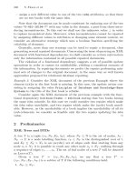
source. The state diagrams of the first-order Markov sources, with their source alphabets having
two and three symbols, are shown in Figure 6.1(a) and (b), respectively. Obviously, an

l

th order
Markov source with

m

symbols in the source alphabet has a total of

m

l

different states. Therefore,
we conclude that a state diagram consists of all the

m

l

states. In the diagram, all the transition
probabilities together with appropriate arrows are used to indicate the state transitions.
The source entropy at a state (

s

i

1

,

s

i

2

,

L

,

s

il

) is defined as
(6.2)
The source entropy is defined as the statistical average of the entropy at all the states. That is,
(6.3)

FIGURE 6.1

State diagrams of the first-order Markov sources with their source alphabets having (a) two
symbols and (b) three symbols.
HSss s psss s psss s
ii
il
ji i
il
j
m
ji i
il
12 12
1
212
,,, ,,, log ,,,LLL
()
=-
()()
=
Â
HS ps s s HSs s s
ii
il
ii
il
ss s S
ii il
l

()
=
()
()
()
Œ
Â
12 12
12
,,, ,,, ,
,,,
LL
L

© 2000 by CRC Press LLC

where, as defined in the previous chapter,

S

l

denotes the

l

th extension of the source alphabet

S

.
That is, the summation is carried out with respect to all

l

-tuples taking over the

S

l

. Extensions of
a Markov source are defined below.

6.1.2 E

XTENSIONS



OF



A

D

ISCRETE

M

ARKOV

S

OURCE

An extension of a Markov source can be defined in a similar way to that of an extension of a
memoryless source in the previous chapter. The definition of extensions of a Markov source and
the relation between the entropy of the original Markov source and the entropy of the

n

th extension
of the Markov source are presented below without derivation. For the derivation, readers are referred
to (Abramson, 1963).

6.1.2.1 Definition

Consider an

l

th order Markov source

S

= {

s

1

,

s

2

,

L

,

s

m

} and a set of conditional probabilities

p

(

s

j

|

s

i

1

,

s

i

2

,

L

,

s

il

), where

j,i

1,

i

2,

L

,

il



Œ

{1,2,

L

,

m

}. Similar to the memoryless source discussed in
Chapter 5, if

n

symbols are grouped into a block, then there is a total of

m

n

blocks. Each block
can be viewed as a new source symbol. Hence, these

m

n

blocks form a new information source
alphabet, called the

n

th extension of the source

S

and denoted by

S

n

. The

n

th extension of the

l

th-
order Markov source is a

k

th-order Markov source, where

k

is the smallest integer greater than or
equal to the ratio between

l

and

n

. That is,
(6.4)
where the notation

Έ

a

Έ

represents the operation of taking the smallest integer greater than or equal
to the quantity

a

.

6.1.2.2 Entropy

Denote, respectively, the entropy of the

lth order Markov source S by H(S), and the entropy of the
nth extension of the lth order Markov source, S
n
, by H(S
n
). The following relation between the two
entropies can be shown:
(6.5)
6.1.3 AUTOREGRESSIVE (AR) MODEL
The Markov source discussed above represents a kind of dependence between source symbols in
terms of the transition probability. Concretely, in determining the transition probability of a present
source symbol given all the previous symbols, only the set of finitely many immediately preceding
symbols matters. The autoregressive model is another kind of dependent source model that has
been used often in image coding. It is defined below.
(6.6)
where s

j
represents the currently observed source symbol, while s
ik
with k = 1,2,L,l denote the l
preceding observed symbols, a
k
’s are coefficients, and x
j
is the current input to the model. If l = 1,
k
l
n
=
È
Í
Í
˘
˙
˙
,
H S nH S
n
()
=
()
sasx
j
kik
j
k

l
=+
=
Â
,
1
© 2000 by CRC Press LLC
the model defined in Equation 6.6 is referred to as the first-order AR model. Clearly, in this case,
the current source symbol is a linear function of its preceding symbol.
6.2 RUN-LENGTH CODING (RLC)
The term run is used to indicate the repetition of a symbol, while the term run-length is used to
represent the number of repeated symbols, in other words, the number of consecutive symbols of
the same value. Instead of encoding the consecutive symbols, it is obvious that encoding the run-
length and the value that these consecutive symbols commonly share may be more efficient. Accord-
ing to an excellent early review on binary image compression by Arps (1979), RLC has been in use
since the earliest days of information theory (Shannon and Weaver, 1949; Laemmel, 1951).
From the discussion of the JPEG in Chapter 4 (with more details in Chapter 7), it is seen that
most of the DCT coefficients within a block of 8 ¥ 8 are zero after certain manipulations. The DCT
coefficients are zigzag scanned. The nonzero DCT coefficients and their addresses in the 8 ¥ 8
block need to be encoded and transmitted to the receiver side. There, the nonzero DCT values are
referred to as labels. The position information about the nonzero DCT coefficients is represented
by the run-length of zeros between the nonzero DCT coefficients in the zigzag scan. The labels
and the run-length of zeros are then Huffman coded.
Many documents such as letters, forms, and drawings can be transmitted using facsimile
machines over the general switched telephone network (GSTN). In digital facsimile techniques,
these documents are quantized into binary levels: black and white. The resolution of these binary
tone images is usually very high. In each scan line, there are many consecutive white and black
pixels, i.e., many alternate white runs and black runs. Therefore it is not surprising to see that RLC
has proven to be efficient in binary document transmission. RLC has been adopted in the interna-
tional standards for facsimile coding: the CCITT Recommendations T.4 and T.6.

RLC using only the horizontal correlation between pixels on the same scan line is referred to
as 1-D RLC. It is noted that the first-order Markov source model with two symbols in the source
alphabet depicted in Figure 6.1(a) can be used to characterize 1-D RLC. To achieve higher coding
efficiency, 2-D RLC utilizes both horizontal and vertical correlation between pixels. Both the 1-D
and 2-D RLC algorithms are introduced below.
6.2.1 1-D RUN-LENGTH CODING
In this technique, each scan line is encoded independently. Each scan line can be considered as a
sequence of alternating, independent white runs and black runs. As an agreement between encoder
and decoder, the first run in each scan line is assumed to be a white run. If the first actual pixel is
black, then the run-length of the first white run is set to be zero. At the end of each scan line, there
is a special codeword called end-of-line (EOL). The decoder knows the end of a scan line when it
encounters an EOL codeword.
Denote run-length by r, which is integer-valued. All of the possible run-lengths construct a
source alphabet R, which is a random variable. That is,
(6.7)
Measurements on typical binary documents have shown that the maximum compression ratio,
z
max
, which is defined below, is about 25% higher when the white and black runs are encoded
separately (Hunter and Robinson, 1980). The average white run-length,
–
r
W
, can be expressed as
(6.8)
Rrr=Œ
{}
:,,,012L
rrPr
WW

r
m
=◊
()
=
Â
0
© 2000 by CRC Press LLC
where m is the maximum value of the run-length, and P
W
(r) denotes the occurrence probability of
a white run with length r. The entropy of the white runs, H
W
, is
(6.9)
For the black runs, the average run-length
–
r
B
and the entropy H
B
can be defined similarly. The
maximum theoretical compression factor z
max
is
(6.10)
Huffman coding is then applied to two source alphabets. According to CCITT Recommendation
T.4, A4 size (210 ¥ 297 mm) documents should be accepted by facsimile machines. In each scan
line, there are 1728 pixels. This means that the maximum run-length for both white and black runs
is 1728, i.e., m = 1728. Two source alphabets of such a large size imply the requirement of two

large codebooks, hence the requirement of large storage space. Therefore, some modification was
made, resulting in the “modified” Huffman (MH) code.
In the modified Huffman code, if the run-length is larger than 63, then the run-length is
represented as
(6.11)
where M takes integer values from 1, 2 to 27, and M ¥ 64 is referred to as the makeup run-length;
T takes integer values from 0, 1 to 63, and is called the terminating run-length. That is, if r £ 63,
the run-length is represented by a terminating codeword only. Otherwise, if r > 63, the run-length
is represented by a makeup codeword and a terminating codeword. A portion of the modified
Huffman code table (Hunter and Robinson, 1980) is shown in Table 6.1. In this way, the requirement
of large storage space is alleviated. The idea is similar to that behind modified Huffman coding,
discussed in Chapter 5.
6.2.2 2-D RUN-LENGTH CODING
The 1-D run-length coding discussed above only utilizes correlation between pixels within a scan
line. In order to utilize correlation between pixels in neighboring scan lines to achieve higher coding
efficiency, 2-D run-length coding was developed. In Recommendation T.4, the modified relative
element address designate (READ) code, also known as the modified READ code or simply the
MR code, was adopted.
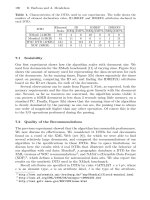
The modified READ code operates in a line-by-line manner. In Figure 6.2, two lines are shown.
The top line is called the reference line, which has been coded, while the bottom line is referred
to as the coding line, which is being coded. There are a group of five changing pixels, a
0
, a
1
, a
2
,
b
1
, b

2
, in the two lines. Their relative positions decide which of the three coding modes is used.
The starting changing pixel a
0
(hence, five changing points) moves from left to right and from top
to bottom as 2-D run-length coding proceeds. The five changing pixels and the three coding modes
are defined below.
6.2.2.1 Five Changing Pixels
By a changing pixel, we mean the first pixel encountered in white or black runs when we scan an
image line-by-line, from left to right, and from top to bottom. The five changing pixels are defined
below.
HPrPr
WWW
r
m
=-
() ()
=
Â
log
2
0
z
max
=
+
+
rr
HH
WB

WB
rM T as r=¥+ >64 63 ,
© 2000 by CRC Press LLC
a
0
: The reference-changing pixel in the coding line. Its position is defined in the previous
coding mode, whose meaning will be explained shortly. At the beginning of a coding
line, a
0
is an imaginary white changing pixel located before the first actual pixel in the
coding line.
a
1
: The next changing pixel in the coding line. Because of the above-mentioned left-to-right
and top-to-bottom scanning order, it is at the right-hand side of a
0
. Since it is a changing
pixel, it has an opposite “color” to that of a
0
.
a
2
: The next changing pixel after a
1
in the coding line. It is to the right of a
1
and has the
same color as that of a
0
.

b
1
: The changing pixel in the reference line that is closest to a
0
from the right and has the
same color as a
1
.
b
2
: The next changing pixel in the reference line after b
1
.
6.2.2.2 Three Coding Modes
Pass Coding Mode — If the changing pixel b
2
is located to the left of the changing pixel a
1
,
it means that the run in the reference line starting from b
1
is not adjacent to the run in the coding
line starting from a
1
. Note that these two runs have the same color. This is called the pass coding
mode. A special codeword, “0001”, is sent out from the transmitter. The receiver then knows that
the run starting from a
0
in the coding line does not end at the pixel below b
2

. This pixel (below b
2
in the coding line) is identified as the reference-changing pixel a
0
of the new set of five changing
pixels for the next coding mode.
Vertical Coding Mode — If the relative distance along the horizontal direction between the
changing pixels a
1
and b
1
is not larger than three pixels, the coding is conducted in vertical coding
FIGURE 6.2 2-D run-length coding.
© 2000 by CRC Press LLC
TABLE 6.1
Modified Huffman Code Table
(Hunter and Robinson, 1980)
Run-
Length White Runs Black Runs
Terminating Codewords
0 00110101 0000110111
1 000111 010
2 0111 11
3 1000 10
4 1011 011
5 1100 0011
6 1110 0010
7 1111 00011
8 10011 000101
Ⅲ

Ⅲ
Ⅲ
Ⅲ
Ⅲ
Ⅲ
Ⅲ
Ⅲ
Ⅲ
Ⅲ
Ⅲ
Ⅲ
60 01001011 000000101100
61 00110010 000001011010
62 00110011 000001100110
63 00110100 000001100111
Makeup Codewords
64 11011 0000001111
128 10010 000011001000
192 010111 000011001001
256 0110111 000001011011
Ⅲ
Ⅲ
Ⅲ
Ⅲ
Ⅲ
Ⅲ
Ⅲ
Ⅲ
Ⅲ
Ⅲ

Ⅲ
Ⅲ
1536 010011001 0000001011010
1600 010011010 0000001011011
1664 011000 0000001100100
1728 010011011 0000001100101
EOL 000000000001 000000000001
TABLE 6.2
2-D Run-Length Coding Table
Mode Conditions Output Codeword Position of New a
0
Pass coding mode b
2
a
1
< 0 0001 Under b
2
in coding line
Vertical coding mode a
1
b
1
= 0 1 a
1
a
1
b
1
= 1 011
a

1
b
1
= 2 000011
a
1
b
1
= 3 0000011
a
1
b
1
= –1 010
a
1
b
1
= –2 000010
a
1
b
1
= –3 0000010
Horizontal coding mode |a
1
b
1
| > 3 001 + (a
0

a
1
) + (a
1
a
2
)a
2
Note: | x
i
y
j
|: distance between x
i
and y
j
, x
i
y
j
> 0: x
i
is right to y
j
, x
i
y
j
< 0: x
i

is left to y
j
.
(x
i
y
j
): codeword of the run denoted by x
i
y
j
taken from the modified Huffman code.
Source: From Hunter and Robinson (1980).
© 2000 by CRC Press LLC
mode. That is, the position of a
1
is coded with reference to the position of b
1
. Seven different
codewords are assigned to seven different cases: the distance between a
1
and b
1
equals 0, ±1, ±2,
±3, where + means a
1
is to the right of b
1
, while – means a
1

is to the left of b
1
. The a
1
then becomes
the reference changing pixel a
0
of the new set of five changing pixels for the next coding mode.
Horizontal Coding Mode — If the relative distance between the changing pixels a
1
and b
1
is
larger than three pixels, the coding is conducted in horizontal coding mode. Here, 1-D run-length
coding is applied. Specifically, the transmitter sends out a codeword consisting the following three
parts: a flag “001”; a 1-D run-length codeword for the run from a
0
to a
1
; a 1-D run-length codeword
for the run from a
1
to a
2
. The a
2
then becomes the reference changing pixel a
0
of the new set of
five changing pixels for the next coding mode. Table 6.2 contains three coding modes and the

corresponding output codewords. There, (a
0
a
1
) and (a
1
a
2
) represent 1-D run-length codewords of
run-length a
0
a
1
and a
1
a
2
, respectively.
6.2.3 EFFECT OF TRANSMISSION ERROR AND UNCOMPRESSED MODE
In this subsection, effect of transmission error in the 1-D and 2-D RLC cases and uncompressed
mode are discussed.
6.2.3.1 Error Effect in the 1-D RLC Case
As introduced above, the special codeword EOL is used to indicate the end of each scan line. With
the EOL, 1-D run-length coding encodes each scan line independently. If a transmission error
occurs in a scan line, there are two possibilities that the effect caused by the error is limited within
the scan line. One possibility is that resynchronization is established after a few runs. One example
is shown in Figure 6.3. There, the transmission error takes place in the second run from the left.
Resynchronization is established in the fifth run in this example. Another possibility lies in the
EOL, which forces resynchronization.
In summary, it is seen that the 1-D run-length coding will not propagate transmission error

between scan lines. In other words, a transmission error will be restricted within a scan line.
Although error detection and retransmission of data via an automatic repeat request (ARQ) system
is supposed to be able to effectively handle the error susceptibility issue, the ARQ technique was
not included in Recommendation T.4 due to the computational complexity and extra transmission
time required.
Once the number of decoded pixels between two consecutive EOL codewords is not equal to
1728 (for an A4 size document), an error has been identified. Some error concealment techniques
can be used to reconstruct the scan line (Hunter and Robinson, 1980). For instance, we can repeat
FIGURE 6.3 Establishment of resynchronization after a few runs.
© 2000 by CRC Press LLC
the previous line, or replace the damaged line by a white line, or use a correlation technique to
recover the line as much as possible.
6.2.3.2 Error Effect in the 2-D RLC Case
From the above discussion, we realize that 2-D RLC is more efficient than 1-D RLC on the one
hand. The 2-D RLC is more susceptible to transmission errors than the 1-D RLC on the other hand.
To prevent error propagation, there is a parameter used in 2-D RLC, known as the K-factor, which
specifies the number of scan lines that are 2-D RLC coded.
Recommendation T.4 defined that no more than K-1 consecutive scan lines be 2-D RLC coded
after a 1-D RLC coded line. For binary documents scanned at normal resolution, K = 2. For
documents scanned at high resolution, K = 4.
According to Arps (1979), there are two different types of algorithms in binary image coding,
raster algorithms and area algorithms. Raster algorithms only operate on data within one or two
raster scan lines. They are hence mainly 1-D in nature. Area algorithms are truly 2-D in nature.
They require that all, or a substantial portion, of the image is in random access memory. From our
discussion above, we see that both 1-D and 2-D RLC defined in T.4 belong to the category of raster
algorithms. Area algorithms require large memory space and are susceptible to transmission noise.
6.2.3.3 Uncompressed Mode
For some detailed binary document images, both 1-D and 2-D RLC may result in data expansion
instead of data compression. Under these circumstances the number of coding bits is larger than
the number of bilevel pixels. An uncompressed mode is created as an alternative way to avoid data

expansion. Special codewords are assigned for the uncompressed mode.
For the performances of 1-D and 2-D RLC applied to eight CCITT test document images, and
issues such as “fill bits” and “minimum scan line time (MSLT),” to name only a few, readers are
referred to an excellent tutorial paper by Hunter and Robinson (1980).
6.3 DIGITAL FACSIMILE CODING STANDARDS
Facsimile transmission, an important means of communication in modern society, is often used as
an example to demonstrate the mutual interaction between widely used applications and standard-
ization activities. Active facsimile applications and the market brought on the necessity for inter-
national standardization in order to facilitate interoperability between facsimile machines world-
wide. Successful international standardization, in turn, has stimulated wider use of facsimile
transmission and, hence, a more demanding market. Facsimile has also been considered as a major
application for binary image compression.
So far, facsimile machines are classified in four different groups. Facsimile apparatuses in
groups 1 and 2 use analog techniques. They can transmit an A4 size (210 ¥ 297 mm) document
scanned at 3.85 lines/mm in 6 and 3 min, respectively, over the GSTN. International standards for
these two groups of facsimile apparatus are CCITT (now ITU) Recommendations T.2 and T.3,
respectively. Group 3 facsimile machines use digital techniques and hence achieve high coding
efficiency. They can transmit the A4 size binary document scanned at a resolution of 3.85 lines/mm
and sampled at 1728 pixels per line in about 1 min at a rate of 4800 b/sec over the GSTN. The
corresponding international standard is CCITT Recommendations T.4. Group 4 facsimile appara-
tuses have the same transmission speed requirement as that for group 3 machines, but the coding
technique is different. Specifically, the coding technique used for group 4 machines is based on
2-D run-length coding, discussed above, but modified to achieve higher coding efficiency. Hence
it is referred to as the modified modified READ coding, abbreviated MMR. The corresponding
standard is CCITT Recommendations T.6. Table 6.3 summarizes the above descriptions.
© 2000 by CRC Press LLC
6.4 DICTIONARY CODING
Dictionary coding, the focus of this section, is different from Huffman coding and arithmetic coding,
discussed in the previous chapter. Both Huffman and arithmetic coding techniques are based on a
statistical model, and the occurrence probabilities play a particular important role. Recall that in

the Huffman coding the shorter codewords are assigned to more frequently occurring source
symbols. In dictionary-based data compression techniques a symbol or a string of symbols generated
from a source alphabet is represented by an index to a dictionary constructed from the source
alphabet. A dictionary is a list of symbols and strings of symbols. There are many examples of this
in our daily lives. For instance, the string “September” is sometimes represented by an index “9,”
while a social security number represents a person in the U.S.
Dictionary coding is widely used in text coding. Consider English text coding. The source
alphabet includes 26 English letters in both lower and upper cases, numbers, various punctuation
marks, and the space bar. Huffman or arithmetic coding treats each symbol based on its occurrence
probability. That is, the source is modeled as a memoryless source. It is well known, however, that
this is not true in many applications. In text coding, structure or context plays a significant role.
As mentioned earlier, it is very likely that the letter u appears after the letter q. Likewise, it is likely
that the word “concerned” will appear after “As far as the weather is.” The strategy of the dictionary
coding is to build a dictionary that contains frequently occurring symbols and string of symbols.
When a symbol or a string is encountered and it is contained in the dictionary, it is encoded with
an index to the dictionary. Otherwise, if not in the dictionary, the symbol or the string of symbols
is encoded in a less efficient manner.
6.4.1 FORMULATION OF DICTIONARY CODING
To facilitate further discussion, we define dictionary coding in a precise manner (Bell et al., 1990).
We denote a source alphabet by S. A dictionary consisting of two elements is defined as D = (P, C),
where P is a finite set of phrases generated from the S, and C is a coding function mapping P onto
a set of codewords.
The set P is said to be complete if any input string can be represented by a series of phrases
chosen from the P. The coding function C is said to obey the prefix property if there is no codeword
that is a prefix of any other codeword. For practical usage, i.e., for reversible compression of any
input text, the phrase set P must be complete and the coding function C must satisfy the prefix property.
6.4.2 CATEGORIZATION OF DICTIONARY-BASED CODING TECHNIQUES
The heart of dictionary coding is the formulation of the dictionary. A successfully built dictionary
results in data compression; the opposite case may lead to data expansion. According to the ways
TABLE 6.3 FACSIMILE CODING STANDARDS

Group of
Facsimile
Apparatuses
Speed
Requirement for
A-4 Size Document
Analog or
Digital Scheme
CCITT
Recommendation
Compression Technique
Model Basic Coder
Algorithm
Acronym
G
1
6 min Analog T.2 — — —
G
2
3 min Analog T.3 — — —
G
3
1 min Digital T.4 1-D RLC
2-D RLC
(optional)
Modified Huffman MH
MR
G
4
1 min Digital T.6 2-D RLC Modified Huffman MMR

© 2000 by CRC Press LLC
in which dictionaries are constructed, dictionary coding techniques can be classified as static or
adaptive.
6.4.2.1 Static Dictionary Coding
In some particular applications, the knowledge about the source alphabet and the related strings of
symbols, also known as phrases, is sufficient for a fixed dictionary to be produced before the coding
process. The dictionary is used at both the transmitting and receiving ends. This is referred to as
static dictionary coding. The merit of the static approach is its simplicity. Its drawbacks lie in its
relatively lower coding efficiency and less flexibility compared with adaptive dictionary techniques.
By less flexibility, we mean that a dictionary built for a specific application is not normally suitable
for utilization in other applications.
An example of static algorithms occurring is digram coding. In this simple and fast coding
technique, the dictionary contains all source symbols and some frequently used pairs of symbols.
In encoding, two symbols are checked at once to see if they are in the dictionary. If so, they are
replaced by the index of the two symbols in the dictionary, and the next pair of symbols is encoded
in the next step. If not, then the index of the first symbol is used to encode the first symbol. The
second symbol is combined with the third symbol to form a new pair, which is encoded in the next
step.
The digram can be straightforwardly extended to n-gram. In the extension, the size of the
dictionary increases and so does its coding efficiency.
6.4.2.2 Adaptive Dictionary Coding
As opposed to the static approach, with the adaptive approach a completely defined dictionary does
not exist prior to the encoding process and the dictionary is not fixed. At the beginning of coding,
only an initial dictionary exists. It adapts itself to the input during the coding process. All the
adaptive dictionary coding algorithms can be traced back to two different original works by Ziv
and Lempel (1977, 1978). The algorithms based on Ziv and Lempel (1977) are referred to as the
LZ77 algorithms, while those based on their 1978 work are the LZ78 algorithms. Prior to intro-
ducing the two landmark works, we will discuss the parsing strategy.
6.4.3 PARSING STRATEGY
Once we have a dictionary, we need to examine the input text and find a string of symbols that

matches an item in the dictionary. Then the index of the item to the dictionary is encoded. This
process of segmenting the input text into disjoint strings (whose union equals the input text) for
coding is referred to as parsing. Obviously, the way to segment the input text into strings is not unique.
In terms of the highest coding efficiency, optimal parsing is essentially a shortest-path problem
(Bell et al., 1990). In practice, however, a method called greedy parsing is used most often. In fact,
it is used in all the LZ77 and LZ78 algorithms. With greedy parsing, the encoder searches for the
longest string of symbols in the input that matches an item in the dictionary at each coding step.
Greedy parsing may not be optimal, but it is simple in its implementation.
Example 6.1
Consider a dictionary, D, whose phrase set P = {a, b, ab, ba, bb, aab, bbb}. The codewords assigned
to these strings are C(a) = 10, C(b) = 11, C(ab) = 010, C(ba) = 0101, C(bb) = 01, C(abb) = 11,
and C(bbb) = 0110. Now the input text is abbaab.
Using greedy parsing, we then encode the text as C(ab).C(ba).C(ab), which is a 10-bit string:
010.0101.010. In the above representations, the periods are used to indicate the division of segments
in the parsing. This, however, is not an optimum solution. Obviously, the following parsing will
be more efficient, i.e., C(a).C(bb).C(aab), which is a 6-bit string: 10.01.11.
© 2000 by CRC Press LLC
6.4.4 SLIDING WINDOW (LZ77) ALGORITHMS
As mentioned earlier, LZ77 algorithms are a group of adaptive dictionary coding algorithms rooted
in the pioneering work of Ziv and Lempel (1977). Since they are adaptive, there is no complete
and fixed dictionary before coding. Instead, the dictionary changes as the input text changes.
6.4.4.1 Introduction
In the LZ77 algorithms, the dictionary used is actually a portion of the input text, which has been
recently encoded. The text that needs to be encoded is compared with the strings of symbols in
the dictionary. The longest matched string in the dictionary is characterized by a pointer (sometimes
called a token), which is represented by a triple of data items. Note that this triple functions as an
index to the dictionary, as mentioned above. In this way, a variable-length string of symbols is
mapped to a fixed-length pointer.
There is a sliding window in the LZ77 algorithms. The window consists of two parts: a search
buffer and a look-ahead buffer. The search buffer contains the portion of the text stream that has

recently been encoded which, as mentioned, is the dictionary; while the look-ahead buffer contains
the text to be encoded next. The window slides through the input text stream from beginning to
end during the entire encoding process. This explains the term sliding window. The size of the
search buffer is much larger than that of the look-ahead buffer. This is expected because what is
contained in the search buffer is in fact the adaptive dictionary. The sliding window is usually on
the order of a few thousand symbols, whereas the look-ahead buffer is on the order of several tens
to one hundred symbols.
6.4.4.2 Encoding and Decoding
Below we present more details about the sliding window dictionary coding technique, i.e., the
LZ77 approach, via a simple illustrative example.
Example 6.2
Figure 6.4 shows a sliding window. The input text stream is ikaccbadaccbaccbaccgikmoabc. In
part (a) of the figure, a search buffer of nine symbols and a look-ahead buffer of six symbols are
shown. All the symbols in the search buffer, accbadacc, have just been encoded. All the symbols
in the look-ahead buffer, baccba, are to be encoded. (It is understood that the symbols before the
FIGURE 6.4 An encoding example using LZ77.
© 2000 by CRC Press LLC
search buffer have been encoded and the symbols after the look-ahead buffer are to be encoded.)
The strings of symbols, ik and ccgikmoabcc, are not covered by the sliding window at the moment.
At the moment, or in other words, in the first step of encoding, the symbol(s) to be encoded
begin(s) with the symbol b. The pointer starts searching for the symbol b from the last symbol in
the search buffer, c, which is immediately to the left of the first symbol b in the look-ahead buffer.
It finds a match at the sixth position from b. It further determines that the longest string of the
match is ba. That is, the maximum matching length is two. The pointer is then represented by a
triple, <i,j,k>. The first item, “i”, represents the distance between the first symbol in the look-ahead
buffer and the position of the pointer (the position of the first symbol of the matched string). This
distance is called offset. In this step, the offset is six. The second item in the triple, “j”, indicates
the length of the matched string. Here, the length of the matched string ba is two. The third item,
“k”, is the codeword assigned to the symbol immediately following the matched string in the look-
ahead buffer. In this step, the third item is C(c), where C is used to represent a function to map

symbol(s) to a codeword, as defined in Section 6.4.1. That is, the resulting triple after the first step
is: <6, 2, C(c)>.
The reason to include the third item “k” into the triple is as follows. In the case where there
is no match in the search buffer, both “i” and “j” will be zero. The third item at this moment is
the codeword of the first symbol in the look-ahead buffer itself. This means that even in the case
where we cannot find a match string, the sliding window still works. In the third step of the encoding
process described below, we will see that the resulting triple is: <0, 0, C(i)>. The decoder hence
understands that there is no matching, and the single symbol i is decoded.
The second step of the encoding is illustrated in part (b) of Figure 6.4. The sliding window has
been shifted to the right by three positions. The first symbol to be encoded now is c, which is the
left-most symbol in the look-ahead buffer. The search pointer moves towards the left from the
symbol c. It first finds a match in the first position with a length of one. It then finds another match
in the fourth position from the first symbol in the look-ahead buffer. Interestingly, the maximum
matching can exceed the boundary between the search buffer and the look-ahead buffer and can
enter the look-ahead buffer. Why this is possible will be seen shortly, when we discuss the decoding
process. In this manner, it is found that the maximum length of matching is five. The last match
is found at the fifth position. The length of the matched string, however, is only one. Since greedy
parsing is used, the match with a length five is chosen. That is, the offset is four and the maximum
match length is five. Consequently, the triple resulting from the second step is <4, 5, C(g)>.
The sliding window is then shifted to the right by six positions. The third step of the encoding
is depicted in Part (c). Obviously, there is no matching of i in the search buffer. The resulting triple
is hence <0, 0, C(i)>.
The encoding process can continue in this way. The possible cases we may encounter in the
encoding, however, are described in the first three steps. Hence we end our discussion of the
encoding process and discuss the decoding process. Compared with the encoding, the decoding is
simpler because there is no need for matching, which involves many comparisons between the
symbols in the look-ahead buffer and the symbols in the search buffer. The decoding process is
illustrated in Figure 6.5.
In the above three steps, the resulting triples are <6, 2, C(c)>, <4, 5, C(g)>, and <0, 0, C(i)>.
Now let us see how the decoder works. That is, how the decoder recovers the string baccbaccgi

from these three triples.
In part (a) of Figure 6.5, the search buffer is the same as that in part (a) of Figure 6.4. That is,
the string accbadacc stored in the search window is what was just decoded.
Once the first triple <6, 2, C(c)> is received, the decoder will move the decoding pointer from
the first position in the look-ahead buffer to the left by six positions. That is, the pointer will point
to the symbol b. The decoder then copies the two symbols starting from b, i.e., ba, into the look-
ahead buffer. The symbol c will be copied right to ba. This is shown in part (b) of Figure 6.5. The
window is then shifted to the right by three positions, as shown in part (c) of Figure 6.5.
© 2000 by CRC Press LLC
After the second triple <4, 5, C(g)> is received, the decoder moves the decoding pointer from
the first position of the look-ahead buffer to the left by four positions. The pointer points to the
symbol c. The decoder then copies five successive symbols starting from the symbol c pointed by
the pointer. We see that at the beginning of this copying process there are only four symbols
available for copying. Once the first symbol is copied, however, all five symbols are available. After
copying, the symbol g is added to the end of the five copied symbols in the look-ahead buffer. The
results are shown in part (c) of Figure 6.5. Part (d) then shows the window shifting to the right by
six positions.
After receiving the triple <0, 0, C(i)>, the decoder knows that there is no match and a single
symbol i is encoded. Hence, the decoder adds the symbol i following the symbol g. This is shown
in part (f) of Figure 6.5.
In Figure 6.5, for each part, the last previously encoded symbol c prior to the receiving of the
three triples is shaded. From part (f), we see that the string added after the symbol c due to the
three triples is baccbaccgi. This agrees with the sequence mentioned at the beginning of our
discussion about the decoding process. We thus conclude that the decoding process has correctly
decoded the encoded sequence from the last encoded symbol and the received triples.
6.4.4.3 Summary of the LZ77 Approach
The sliding window consists of two parts: the search buffer and the look-ahead buffer. The most
recently encoded portion of the input text stream is contained in the search buffer, while the portion
of the text that needs to be encoded immediately is in the look-ahead buffer. The first symbol in
the look-ahead buffer, located to the right of the boundary between the two buffers, is the symbol

FIGURE 6.5 A decoding example using LZ77.
© 2000 by CRC Press LLC
or the beginning of a string of symbols to be encoded at the moment. Let us call it the symbol s.
The size of the search buffer is usually much larger than that of the look-ahead buffer.
In encoding, the search pointer moves to the left, away from the symbol s, to find a match of
the symbol s in the search buffer. Once a match is found, the encoding process will further determine
the length of the matched string. When there are multiple matches, the match that produces the
longest matched string is chosen. The match is denoted by a triple <i, j, k>. The first item in the
triple, “i”, is the offset, which is the distance between the pointer pointing to the symbol giving
the maximum match and the symbol s. The second item, “j”, is the length of the matched string.
The third item, “k”, is the codeword of the symbol following the matched string in the look-ahead
buffer. The sliding window is then shifted to the right by j+1 positions before the next coding step
takes place.
When there is no matching in the search buffer, the triple is represented by <0, 0, C(s)>, where
C(s) is the codeword assigned to the symbol s. The sliding window is then shifted to the right by
one position.
The sliding window is shifted along the input text stream during the encoding process. The
symbol s moves from the beginning symbol to the ending symbol of the input text stream.
At the very beginning, the content of the search buffer can be arbitrarily selected. For instance,
the symbols in the search buffer may all be the space symbol.
Let us denote the size of the search buffer by SB, the size of the look-ahead buffer by L, and
the size of the source alphabet by A. Assume that the natural binary code is used. Then we see that
the LZ77 approach encodes variable-length strings of symbols with fixed-length codewords. Spe-
cifically, the offset “i” is of coding length Έ log
2
SB Έ, the length of matched string “j” is of coding
length Έ log
2
(SB + L) Έ, and the codeword “k” is of coding length Έ log
2

(A) Έ, where the sign
denotes the smallest integer larger than a.
The length of the matched string is equal to Έ log
2
(SB + L) Έ because the search for the maximum
matching can enter into the look-ahead buffer as shown in Example 6.2.
The decoding process is simpler than the encoding process since there are no comparisons
involved in the decoding.
The most recently encoded symbols in the search buffer serve as the dictionary used in the
LZ77 approach. The merit of doing so is that the dictionary is well adapted to the input text. The
limitation of the approach is that if the distance between the repeated patterns in the input text
stream is larger than the size of the search buffer, then the approach cannot utilize the structure to
compress the text. A vivid example can be found in (Sayood, 1996).
A window with a moderate size, say, SB + L £ 8192, can compress a variety of texts well.
Several reasons have been analyzed by Bell et al. (1990).
Many variations have been made to improve coding efficiency of the LZ77 approach. The LZ77
produces a triple in each encoding step; i.e., the offset (position of the matched string), the length
of the matched string, and the codeword of the symbol following the matched string. The trans-
mission of the third item in each coding step is not efficient. This is true especially at the beginning
of coding. A variant of the LZ77, referred to as the LZSS algorithm, improves this inefficiency.
6.4.5 LZ78 ALGORITHMS
6.4.5.1 Introduction
As mentioned above, the LZ77 algorithms use a sliding window of fixed size, and both the search
buffer and the look-ahead buffer have a fixed size. This means that if the distance between two
repeated patterns is larger than the size of the search buffer, the LZ77 algorithms cannot work
efficiently. The fixed size of both the buffers implies that the matched string cannot be longer than
the sum of the sizes of the two buffers, placing another limitation on coding efficiency. Increasing
the sizes of the search buffer and the look-ahead buffer seemingly will resolve the problem. A close
a
© 2000 by CRC Press LLC

look, however, reveals that it also leads to increases in the number of bits required to encode the
offset and matched string length, as well as an increase in processing complexity.
The LZ78 algorithms (Ziv and Lempel, 1978) eliminate the use of the sliding window. Instead,
these algorithms use the encoded text as a dictionary which, potentially, does not have a fixed size.
Each time a pointer (token) is issued, the encoded string is included in the dictionary. Theoretically,
the LZ78 algorithms reach optimal performance as the encoded text stream approaches infinity. In
practice, however, as mentioned above with respect to the LZ77, a very large dictionary will affect
coding efficiency negatively. Therefore, once a preset limit to the dictionary size has been reached,
either the dictionary is fixed for the future (if the coding efficiency is good), or it is reset to zero,
i.e., it must be restarted.
Instead of the triples used in the LZ77, only pairs are used in the LZ78. Specifically, only the
position of the pointer to the matched string and the symbol following the matched string need to
be encoded. The length of the matched string does not need to be encoded since both the encoder
and the decoder have exactly the same dictionary, i.e., the decoder knows the length of the matched
string.
6.4.5.2 Encoding and Decoding
Like the discussion of the LZ77 algorithms, we will go through an example to describe the LZ78
algorithms.
Example 6.3
Consider the text stream: baccbaccacbcabccbbacc. Table 6.4 shows the coding process. We see
that for the first three symbols there is no match between the individual input symbols and the
entries in the dictionary. Therefore, the doubles are, respectively, <0, C(b)>, <0, C(a)>, and
<0, C(c)>, where 0 means no match, and C(b), C(a), and C(c) represent the codewords of b, a, and
c, respectively. After symbols b, a, c, comes c, which finds a match in the dictionary (the third
entry). Therefore, the next symbol b is combined to be considered. Since the string cb did not
appear before, it is encoded as a double and it is appended as a new entry into the dictionary. The
first item in the double is the index of the matched entry c, 3, the second item is the index/codeword
of the symbol following the match b, 1. That is, the double is <3, 1>. The following input symbol
is a, which appeared in the dictionary. Hence, the next symbol c is taken into consideration. Since
the string ac is not an entry of the dictionary, it is encoded with a double. The first item in the

double is the index of symbol a, 2; the second item is the index of symbol c, 3, i.e., <2, 3>. The
encoding proceeds in this way. Take a look at Table 6.4. In general, as the encoding proceeds, the
entries in the dictionary become longer and longer. First, entries with single symbols come out,
but later, more and more entries with two symbols show up. After that, more and more entries with
three symbols appear. This means that coding efficiency is increasing.
Now consider the decoding process. Since the decoder knows the rule applied in the encoding,
it can reconstruct the dictionary and decode the input text stream from the received doubles. When
the first double <0, C(b)> is received, the decoder knows that there is no match. Hence, the first
entry in the dictionary is b. So is the first decoded symbol. From the second double <0, C(a)>,
symbol a is known as the second entry in the dictionary as well as the second decoded symbol.
Similarly, the next entry in the dictionary and the next decoded symbol are known as c. When the
following double <3, 1> is received. The decoder knows from two items, 3 and 1, that the next
two symbols are the third and the first entries in the dictionary. This indicates that the symbols c
and b are decoded, and the string cb becomes the fourth entry in the dictionary.
We omit the next two doubles and take a look at the double <4, 3>, which is associated with
Index 7 in Table 6.4. Since the first item in the double is 4, it means that the maximum matched
string is cb, which is associated with Index 4 in Table 6.4. The second item in the double, 3, implies
that the symbol following the match is the third entry c. Therefore the decoder decodes a string
cbc. Also the string cbc becomes the seventh entry in the reconstructed dictionary. In this way, the
© 2000 by CRC Press LLC
decoder can reconstruct the exact same dictionary as that established by the encoder and decode
the input text stream from the received doubles.
6.4.5.3 LZW Algorithm
Both the LZ77 and LZ78 approaches, when published in 1977 and 1978, respectively, were theory
oriented. The effective and practical improvement over the LZ78 by Welch (1984) brought much
attention to the LZ dictionary coding techniques. The resulting algorithm is referred to the LZW
algorithm. It removed the second item in the double (the index of the symbol following the longest
matched string) and, hence, it enhanced coding efficiency. In other words, the LZW only sends the
indexes of the dictionary to the decoder. For the purpose, the LZW first forms an initial dictionary,
which consists of all the individual source symbols contained in the source alphabet. Then, the

encoder examines the input symbol. Since the input symbol matches to an entry in the dictionary,
its succeeding symbol is cascaded to form a string. The cascaded string does not find a match in
the initial dictionary. Hence, the index of the matched symbol is encoded and the enlarged string
(the matched symbol followed by the cascaded symbol) is listed as a new entry in the dictionary.
The encoding process continues in this manner.
For the encoding and decoding processes, let us go through an example to see how the LZW
algorithm can encode only the indexes and the decoder can still decode the input text string.
Example 6.4
Consider the following input text stream: accbadaccbaccbacc. We see that the source alphabet is
S = {a,b,c,d,}. The top portion of Table 6.5 (with indexes 1,2,3,4) gives a possible initial dictionary
used in the LZW. When the first symbol a is input, the encoder finds that it has a match in the
dictionary. Therefore the next symbol c is taken to form a string ac. Because the string ac is not
in the dictionary, it is listed as a new entry in the dictionary and is given an index, 5. The index
of the matched symbol a, 1, is encoded. When the second symbol, c, is input the encoder takes
the following symbol c into consideration because there is a match to the second input symbol c
in the dictionary. Since the string cc does not match any existing entry, it becomes a new entry in
the dictionary with an index, 6. The index of the matched symbol (the second input symbol), c, is
encoded. Now consider the third input symbol c, which appeared in the dictionary. Hence, the
following symbol b is cascaded to form a string cb. Since the string cb is not in the dictionary, it
becomes a new entry in the dictionary and is given an index, 7. The index of matched symbol c, 3,
is encoded. The process proceeds in this fashion.
TABLE 6.4
An Encoding Example Using the LZ78 Algorithm
Index Doubles Encoded Symbols
1 < 0, C(b) > b
2 < 0, C(a) > a
3 < 0, C(c) > c
4 < 3, 1 > cb
5 < 2, 3 > ac
6 < 3, 2 > ca

7 < 4, 3 > cbc
8 < 2, 1 > ab
9 < 3, 3 > cc
10 < 1, 1 > bb
11 < 5, 3 > acc
© 2000 by CRC Press LLC
Take a look at entry 11 in the dictionary shown in Table 6.5. The input symbol at this point is
a. Since it has a match in the previous entries, its next symbol c is considered. Since the string ac
appeared in entry 5, the succeeding symbol c is combined. Now the new enlarged string becomes
acc and it does not have a match in the previous entries. It is thus added to the dictionary. And a
new index, 11, is given to the string acc. The index of the matched string ac, 5, is encoded and
transmitted. The final sequence of encoded indexes is 1, 3, 3, 2, 1, 4, 5, 7, 11, 8. Like the LZ78,
the entries in the dictionary become longer and longer in the LZW algorithm. This implies high
coding efficiency since long strings can be represented by indexes.
Now let us take a look at the decoding process to see how the decoder can decode the input
text stream from the received index. Initially, the decoder has the same dictionary (the top four
rows in Table 6.5) as that in the encoder. Once the first index 1 comes, the decoder decodes a
symbol a. The second index is 3, which indicates that the next symbol is c. From the rule applied
in encoding, the decoder knows further that a new entry ac has been added to the dictionary with
an index 5. The next index is 3. It is known that the next symbol is also c. It is also known that
the string cc has been added into the dictionary as the sixth entry. In this way, the decoder
reconstructs the dictionary and decodes the input text stream.
6.4.5.4 Summary
The LZW algorithm, as a representative of the LZ78 approach, is summarized below.
The initial dictionary contains the indexes for all the individual source symbols. At the beginning
of encoding, when a symbol is input, since it has a match in the initial dictionary, the next symbol
is cascaded to form a two-symbol string. Since the two-symbol string cannot find a match in the
initial dictionary, the index of the former symbol is encoded and transmitted, and the two-symbol
string is added to the dictionary with a new, incremented index. The next encoding step starts with
the latter symbol of the two.

In the middle, the encoding process starts with the last symbol of the latest added dictionary
entry. Since it has a match in the previous entries, its succeeding symbol is cascaded after the
symbol to form a string. If this string appeared before in the dictionary (i.e., the string finds a
TABLE 6.5
An Example of the Dictionary Coding
Using the LZW Algorithm
Index Entry Input Symbols
Encoded
Index
1a
Initial dictionary
2b
3c
4d
5ac a 1
6cc c 3
7cb c 3
8ba b 2
9ad a 1
10 da d 4
11 acc a,c 5
12 cba c,b 7
13 accb a,c,c 11
14 bac b,a, 8
15 cc… c,c,…
¸
˝
Ô
˛
Ô

© 2000 by CRC Press LLC
match), the next symbol is cascaded as well. This process continues until such an enlarged string
cannot find a match in the dictionary. At this moment, the index of the last matched string (the
longest match) is encoded and transmitted, and the enlarged and unmatched string is added into
the dictionary as a new entry with a new, incremented index.
Decoding is a process of transforming the index string back to the corresponding symbol string.
In order to do so, however, the dictionary must be reconstructed in exactly the same way as that
established in the encoding process. That is, the initial dictionary is constructed first in the same
way as that in the encoding. When decoding the index string, the decoder reconstructs the same
dictionary as that in the encoder according to the rule used in the encoding.
Specifically, at the beginning of the decoding, after receiving an index, a corresponding single
symbol can be decoded. Via the next received index, another symbol can be decoded. From the
rule used in the encoding, the decoder knows that the two symbols should be cascaded to form a
new entry added into the dictionary with an incremented index. The next step in the decoding will
start from the latter symbol among the two symbols.
Now consider the middle of the decoding process. The presently received index is used to
decode a corresponding string of input symbols according to the reconstructed dictionary at the
moment. (Note that this string is said to be with the present index.) It is known from the encoding
rule that the symbols in the string associated with the next index should be considered. (Note that
this string is said to be with the next index.) That is, the first symbol in the string with the next
index should be appended to the last symbol in the string with the present index. The resultant
combination, i.e., the string with the present index followed by the first symbol in the string with
the next index, cannot find a match to an entry in the dictionary. Therefore, the combination should
be added to the dictionary with an incremented index. At this moment, the next index becomes the
new present index, and the index following the next index becomes the new next index. The decoding
process then proceeds in the same fashion in a new decoding step.
Compared with the LZ78 algorithm, the LZW algorithm eliminates the necessity of having the
second item in the double, an index/codeword of the symbol following a matched string. That is,
the encoder only needs to encode and transmit the first item in the double. This greatly enhances
the coding efficiency and reduces the complexity of the LZ algorithm.

6.4.5.5 Applications
The CCITT Recommendation V.42 bis is a data compression standard used in modems that connect
computers with remote users via the GSTN. In the compressed mode, the LZW algorithm is
recommended for data compression.
In image compression, the LZW finds its application as well. Specifically, it is utilized in the
graphic interchange format (GIF) which was created to encode graphical images. GIF is now also
used to encode natural images, though it is not very efficient in this regard. For more information,
readers are referred to Sayood (1996). The LZW algorithm is also used in the UNIX Compress
command.
6.5 INTERNATIONAL STANDARDS FOR LOSSLESS STILL
IMAGE COMPRESSION
In the previous chapter, we studied Huffman and arithmetic coding techniques. We also briefly
discussed the international standard for bilevel image compression, known as the JBIG. In this
chapter, so far we have discussed another two coding techniques: the run-length and dictionary
coding techniques. We also introduced the international standards for facsimile compression, in
which the techniques known as the MH, MR, and MMR were recommended. All of these techniques
involve lossless compression. In the next chapter, the international still image coding standard JPEG
will be introduced. As we will see, the JPEG has four different modes. They can be divided into
© 2000 by CRC Press LLC
two compression categories: lossy and lossless. Hence, we can talk about the lossless JPEG. Before
leaving this chapter, however, we briefly discuss, compare, and summarize various techniques used
in the international standards for lossless still image compression. For more details, readers are
referred to an excellent survey paper by Arps and Truong (1994).
6.5.1 LOSSLESS BILEVEL STILL IMAGE COMPRESSION
6.5.1.1 Algorithms
As mentioned above, there are four different international standard algorithms falling into this
category.
MH (Modified Huffman coding) — This algorithm is defined in CCITT Recommendation
T.4 for facsimile coding. It uses the 1-D run-length coding technique followed by the “modified”
Huffman coding technique.

MR (Modified READ [Relative Element Address Designate] coding) — Defined in CCITT
Recommendation T.4 for facsimile coding. It uses the 2-D run-length coding technique followed
by the “modified” Huffman coding technique.
MMR (Modified Modified READ coding) — Defined in CCITT Recommendation T.6. It is
based on MR, but is modified to maximize compression.
JBIG (Joint Bilevel Image experts Group coding) — Defined in CCITT Recommendation
T.82. It uses an adaptive 2-D coding model, followed by an adaptive arithmetic coding technique.
6.5.1.2 Performance Comparison
The JBIG test image set was used to compare the performance of the above-mentioned algorithms.
The set contains scanned business documents with different densities, graphic images, digital
halftones, and mixed (document and halftone) images.
Note that digital halftones, also named (digital) halftone images, are generated by using only
binary devices. Some small black units are imposed on a white background. The units may assume
different shapes: a circle, a square, and so on. The more dense the black units in a spot of an image,
the darker the spot appears. The digital halftoning method has been used for printing gray-level
images in newspapers and books. Digital halftoning through character overstriking, used to generate
digital images in the early days for the experimental work associated with courses on digital image
processing, has been described by Gonzalez and Woods (1992).
The following two observations on the performance comparison were made after the application
of the several techniques to the JBIG test image set.
1. For bilevel images excluding digital halftones, the compression ratio achieved by these
techniques ranges from 3 to 100. The compression ratio increases monotonically in the
order of the following standard algorithms: MH, MR, MMR, JBIG.
2. For digital halftones, MH, MR, and MMR result in data expansion, while JBIG achieves
compression ratios in the range of 5 to 20. This demonstrates that among the techniques,
JBIG is the only one suitable for the compression of digital halftones.
6.5.2 LOSSLESS MULTILEVEL STILL IMAGE COMPRESSION
6.5.2.1 Algorithms
There are two international standards for multilevel still image compression:
JBIG (Joint Bilevel Image experts Group coding) — Defined in CCITT Recommendation

T.82. It uses an adaptive arithmetic coding technique. To encode multilevel images, the JIBG
decomposes multilevel images into bit-planes, then compresses these bit-planes using its bilevel
© 2000 by CRC Press LLC
image compression technique. To further enhance the compression ratio, it uses Gary coding to
represent pixel amplitudes instead of weighted binary coding.
JPEG (Joint Photographic (image) Experts Group coding) — Defined in CCITT Recom-
mendation T.81. For lossless coding, it uses the differential coding technique. The predictive error
is encoded using either Huffman coding or adaptive arithmetic coding techniques.
6.5.2.2 Performance Comparison
A set of color test images from the JPEG standards committee was used for performance compar-
ison. The luminance component (Y) is of resolution 720 ¥ 576 pixels, while the chrominance
components (U and V) are of 360 ¥ 576 pixels. The compression ratios calculated are the combined
results for all the three components. The following observations have been reported.
1. When quantized in 8 bits per pixel, the compression ratios vary much less for multilevel
images than for bilevel images, and are roughtly equal to 2.
2. When quantized with 5 bits per pixel down to 2 bits per pixel, compared with the lossless
JPEG the JBIG achieves an increasingly higher compression ratio, up to a maximum of
29%.
3. When quantized with 6 bits per pixel, JBIG and lossless JPEG achieve similar compres-
sion ratios.
4. When quantized with 7 bits per pixel to 8 bits per pixel, the lossless JPEG achieves a
2.4 to 2.6% higher compression ratio than JBIG.
6.6 SUMMARY
Both Huffman coding and arithmetic coding, discussed in the previous chapter, are referred to as
variable-length coding techniques, since the lengths of codewords assigned to different entries in
a source alphabet are different. In general, a codeword of a shorter length is assigned to an entry
with higher occurrence probabilities. They are also classified as fixed-length to variable-length
coding techniques (Arps, 1979), since the entries in a source alphabet have the same fixed length.
Run-length coding (RLC) and dictionary coding, the focus of this chapter, are opposite, and are
referred to as variable-length to fixed-length coding techniques. This is because the runs in the

RLC and the string in the dictionary coding are variable and are encoded with codewords of the
same fixed length.
Based on RLC, the international standard algorithms for facsimile coding, MH, MR, and MMR
have worked successfully except for dealing with digital halftones. That is, these algorithms result
in data expansion when applied to digital halftones. The JBIG, based on an adaptive arithmetic
coding technique, not only achieves a higher coding efficiency than MH, MR, and MMR for
facsimile coding, but also compresses the digital halftones effectively.
Note that 1-D RLC utilizes the correlation between pixels within a scan line, whereas 2-D RLC
utilizes the correlation between pixels within a few scan lines. As a result, 2-D RLC can obtain
higher coding efficiency than 1-D RLC. On the other hand, 2-D RLC is more susceptible to
transmission errors than 1-D RLC.
In text compression, the dictionary-based techniques have proven to be efficient. All the adaptive
dictionary-based algorithms can be classified into two groups. One is based on a work by Ziv and
Lempel in 1977, and another is based on their pioneering work in 1978. They are called the LZ77
and LZ78 algorithms, respectively. With the LZ77 algorithms, a fixed-size window slides through
the input text stream. The sliding window consists of two parts: the search buffer and the look-
ahead buffer. The search buffer contains the most recently encoded portion of the input text, while
the look-ahead buffer contains the portion of the input text to be encoded immediately. For the
symbols to be encoded, the LZ77 algorithms search for the longest match in the search buffer. The
© 2000 by CRC Press LLC
information about the match: the distance between the matched string in the search buffer and that
in the look-ahead buffer, the length of the matched string, and the codeword of the symbol following
the matched string in the look-ahead buffer are encoded. Many improvements have been made in
the LZ77 algorithms.
The performance of the LZ77 algorithms is limited by the sizes of the search buffer and the
look-ahead buffer. With a finite size for the search buffer, the LZ77 algorithms will not work well
in the case where repeated patterns are apart from each other by a distance longer than the size of
the search buffer. With a finite size for the sliding window, the LZ77 algorithms will not work well
in the case where matching strings are longer than the window. In order to be efficient, however,
these sizes cannot be very large.

In order to overcome the problem, the LZ78 algorithms work in a different way. They do not
use the sliding window at all. Instead of using the most recently encoded portion of the input text
as a dictionary, the LZ78 algorithms use the index of the longest matched string as an entry of the
dictionary. That is, each matched string cascaded with its immediate next symbol is compared with
the existing entries of the dictionary. If this combination (a new string) does not find a match in
the dictionary constructed at the moment, the combination will be included as an entry in the
dictionary. Otherwise, the next symbol in the input text will be appended to the combination and
the enlarged new combination will be checked with the dictionary. The process continues until the
new combination cannot find a match in the dictionary. Among the several variants of the LZ78
algorithms, the LZW algorithm is perhaps the most important one. It only needs to encode the
indexes of the longest matched strings to the dictionary. It can be shown that the decoder can
decode the input text stream from the given index stream. In doing so, the same dictionary as that
established in the encoder needs to be reconstructed at the decoder, and this can be implemented
since the same rule used in the encoding is known in the decoder.
The size of the dictionary cannot be infinitely large because, as mentioned above, the coding
efficiency will not be high. The common practice of the LZ78 algorithms is to keep the dictionary
fixed once a certain size has been reached and the performance of the encoding is satisfactory.
Otherwise, the dictionary will be set to empty and will be reconstructed from scratch.
Considering the fact that there are several international standards concerning still image coding
(for both bilevel and multilevel images), a brief summary of them and a performance comparison
have been presented in this chapter. At the beginning of this chapter, a description of the discrete
Markov source and its nth extensions was provided. The Markov source and the autoregressive
model serve as important models for the dependent information sources.
6.7 EXERCISES
6-1. Draw the state diagram of a second-order Markov source with two symbols in the source
alphabet. That is, S = {s
1
, s
2
}. It is assumed that the conditional probabilities are

6-2. What are the definitions of raster algorithm and area algorithm in binary image coding?
To which category does 1-D RLC belong? To which category does 2-D RLC belong?
6-3. What effect does a transmission error have on 1-D RLC and 2-D RLC, respectively?
What is the function of the codeword EOL?
ps ss ps ss
ps ss ps ss
ps ss ps ss ps ss ps ss
111 222
211 122
1 12 1 21 2 12 2 21
07
03
05
()
=
()
=
()
=
()
=
()
=
()
=
()
=
()
=
.,

.,

and
© 2000 by CRC Press LLC
6-4. Make a convincing argument that the “modified” Huffman (MH) algorithm reduces the
requirement of large storage space.
6-5. Which three different modes does 2-D RLC have? How do you view the vertical mode?
6-6. Using your own words, describe the encoding and decoding processes of the LZ77
algorithms. Go through Example 6.2.
6-7. Using your own words, describe the encoding and decoding processes of the LZW
algorithm. Go through Example 6.3.
6-8. Read the reference paper (Arps and Truong, 1994), which is an excellent survey on the
international standards for lossless still image compression. Pay particular attention to
all the figures and to Table 1.
REFERENCES
Abramson, N. Information Theory and Coding, New York: McGraw-Hill, 1963.
Arps, R. B. Binary Image Compression, in Image Transmission Techniques, W. K. Pratt (Ed.), New York:
Academic Press, 1979.
Arps, R. B. and T. K. Truong, Comparison of international standards for lossless still image compression,
Proc. IEEE, 82(6), 889-899, 1994.
Bell, T. C., J. G. Cleary, and I. H. Witten, Text Compression, Englewood Cliffs, NJ: Prentice-Hall, 1990.
Gonzalez, R. C. and R. E. Woods, Digital Image Processing, Reading, MA: Addison-Wesley, 1992.
Hunter, R. and A. H. Robinson, International digital facsimile coding standards, Proc. IEEE, 68(7), 854-867,
1980.
Laemmel, A. E. Coding Processes for Bandwidth Reduction in Picture Transmission, Rep. R-246-51, PIB-
187, Microwave Res. Inst., Polytechnic Institute of Brooklyn, New York.
Nelson, M. and J L. Gailly, The Data Compression Book, 2nd ed., New York: M&T Books, 1995.
Sayood, K. Introduction to Data Compression, San Francisco, CA: Morgan Kaufmann Publishers, 1996.
Shannon, C. E. and W. Weaver, The Mathematical Theory of Communication, Urbana, IL: University of Illinois
Press, 1949.

Welch, T. A technique for high-performance data compression, IEEE Trans. Comput., 17(6), 8-19, 1984.
Ziv, J. and A. Lempel, A universal algorithm for sequential data compression, IEEE Trans. Inf. Theory, 23(3),
337-343, 1977.
Ziv, J. and A. Lempel, Compression of individual sequences via variable-rate coding, IEEE Trans. Inf. Theory,
24(5), 530-536, 1978.