Tài liệu Advanced DSP and Noise reduction P4 pptx
Bạn đang xem bản rút gọn của tài liệu. Xem và tải ngay bản đầy đủ của tài liệu tại đây (569 KB, 54 trang )
4
BAYESIAN ESTIMATION
4.1 Bayesian Estimation Theory: Basic Definitions
4.2 Bayesian Estimation
4.3 The Estimate–Maximise Method
4.4 Cramer–Rao Bound on the Minimum Estimator Variance
4.5
Design of Mixture Gaussian Models
4.6 Bayesian Classification
4.7 Modeling the Space of a Random Process
4.8
Summary
ayesian estimation is a framework for the formulation of statistical
inference problems. In the prediction or estimation of a random
process from a related observation signal, the Bayesian philosophy is
based on combining the evidence contained in the signal with prior
knowledge of the probability distribution of the process. Bayesian
methodology includes the classical estimators such as maximum a posteriori
(MAP), maximum-likelihood (ML), minimum mean square error (MMSE)
and minimum mean absolute value of error (MAVE) as special cases. The
hidden Markov model, widely used in statistical signal processing, is an
example of a Bayesian model. Bayesian inference is based on minimisation
of the so-called Bayes’ risk function, which includes a posterior model of
the unknown parameters given the observation and a cost-of-error function.
This chapter begins with an introduction to the basic concepts of estimation
theory, and considers the statistical measures that are used to quantify the
performance of an estimator. We study Bayesian estimation methods and
consider the effect of using a prior model on the mean and the variance of an
estimate. The estimate–maximise (EM) method for the estimation of a set of
unknown parameters from an incomplete observation is studied, and applied
to the mixture Gaussian modelling of the space of a continuous random
variable. This chapter concludes with an introduction to the Bayesian
classification of discrete or finite-state signals, and the K-means clustering
method.
B
f(y,
θ)
f(
θ
|
y
1
)
1
y
y
θ
f(
θ
|
y
2
)
2
y
Advanced Digital Signal Processing and Noise Reduction, Second Edition.
Saeed V. Vaseghi
Copyright © 2000 John Wiley & Sons Ltd
ISBNs: 0-471-62692-9 (Hardback): 0-470-84162-1 (Electronic)
90
Bayesian Estimation
4.1 Bayesian Estimation Theory: Basic Definitions
Estimation theory is concerned with the determination of the best estimate
of an unknown parameter vector from an observation signal, or the recovery
of a clean signal degraded by noise and distortion. For example, given a
noisy sine wave, we may be interested in estimating its basic parameters
(i.e. amplitude, frequency and phase), or we may wish to recover the signal
itself. An estimator takes as the input a set of noisy or incomplete
observations, and, using a dynamic model (e.g. a linear predictive model)
and/or a probabilistic model (e.g. Gaussian model) of the process, estimates
the unknown parameters. The estimation accuracy depends on the available
information and on the efficiency of the estimator. In this chapter, the
Bayesian estimation of continuous-valued parameters is studied. The
modelling and classification of finite-state parameters is covered in the next
chapter.
Bayesian theory is a general inference framework. In the estimation or
prediction of the state of a process, the Bayesian method employs both the
evidence contained in the observation signal and the accumulated prior
probability of the process. Consider the estimation of the value of a random
parameter vector
θ
, given a related observation vector y. From Bayes’ rule
the posterior probability density function (pdf) of the parameter vector
θ
given y,
f
Θ
|
Y
(
θ
|
y
)
, can be expressed as
)(
)()|(
)|(
|
y
y
y
Y
|Y
Y
f
ff
f
θθ
θ
ΘΘ
Θ
=
(4.1)
where for a given observation, f
Y
(y) is a constant and has only a normalising
effect. Thus there are two variable terms in Equation (4.1): one term
f
Y
|
Θ
(y|
θ
) is the likelihood that the observation signal y was generated by the
parameter vector
θ
and the second term is the prior probability of the
parameter vector having a value of
θ
. The relative influence of the
likelihood pdf f
Y
|
Θ
(y|
θ
) and the prior pdf f
Θ
(
θ
) on the posterior pdf f
Θ
|
Y
(
θ
|y)
depends on the shape of these function, i.e. on how relatively peaked each
pdf is. In general the more peaked a probability density function, the more it
will influence the outcome of the estimation process. Conversely, a uniform
pdf will have no influence.
The remainder of this chapter is concerned with different forms of Bayesian
estimation and its applications. First, in this section, some basic concepts of
estimation theory are introduced.
Basic Definitions
91
4.1.1 Dynamic and Probability Models in Estimation
Optimal estimation algorithms utilise dynamic and statistical models of the
observation signals. A dynamic predictive model captures the correlation
structure of a signal, and models the dependence of the present and future
values of the signal on its past trajectory and the input stimulus. A statistical
probability model characterises the random fluctuations of a signal in terms
of its statistics, such as the mean and the covariance, and most completely in
terms of a probability model. Conditional probability models, in addition to
modelling the random fluctuations of a signal, can also model the
dependence of the signal on its past values or on some other related process.
As an illustration consider the estimation of a P-dimensional parameter
vector
θ
=[
θ
0
,
θ
1
, ,
θ
P
–1
] from a noisy observation vector y=[y(0), y(1), ,
y(N–1)] modelled as
nex
y
+=
)(
,,h
θ
(4.2)
where, as illustrated in Figure 4.1, the function h(·) with a random input e,
output x, and parameter vector
θ
, is a predictive model of the signal x, and n
is an additive random noise process. In Figure 4.1, the distributions of the
random noise n, the random input e and the parameter vector
θ
are modelled
by probability density functions, f
N
(n), f
E
(e), and f
Θ
(
θ
) respectively. The pdf
model most often used is the Gaussian model. Predictive and statistical
models of a process guide the estimator towards the set of values of the
unknown parameters that are most consistent with both the prior distribution
of the model parameters and the noisy observation. In general, the more
modelling information used in an estimation process, the better the results,
provided that the models are an accurate characterisation of the observation
and the parameter process.
x
y
=
x
+
n
Excitation process
f
E
(
e
)
Noise process
e
Predictive model
Parameter process
θ
n
f
Θ Θ
(
θ
)
f
N
(
n
)
h
Θ Θ
(
θ
,
x
,
e
)
Figure 4.1
A random process
y
is described in terms of a predictive model
h
(
·
),
and statistical models
f
E
(
·
),
f
Θ
(
·
) and
f
N
(
·
).
92
Bayesian Estimation
4.1.2 Parameter Space and Signal Space
Consider a random process with a parameter vector
θ
. For example, each
instance of
θ
could be the parameter vector for a dynamic model of a speech
sound or a musical note. The parameter space of a process
Θ
is the
collection of all the values that the parameter vector
θ
can assume. The
parameters of a random process determine the “character” (i.e. the mean, the
variance, the power spectrum, etc.) of the signals generated by the process.
As the process parameters change, so do the characteristics of the signals
generated by the process. Each value of the parameter vector
θ
of a process
has an associated signal space Y; this is the collection of all the signal
realisations of the process with the parameter value
θ
. For example,
consider a three-dimensional vector-valued Gaussian process with parameter
vector
θ
=[
µ
,
Σ
], where
µ
is the mean vector and
Σ
is the covariance matrix
of the Gaussian process. Figure. 4.2 illustrates three mean vectors in a three-
dimensional parameter space. Also shown is the signal space associated
with each parameter. As shown, the signal space of each parameter vector of
a Gaussian process contains an infinite number of points, centred on the
mean vector
µ
, and with a spatial volume and orientation that are
determined by the covariance matrix
Σ
.
For simplicity, the variances are not
shown in the parameter space, although they are evident in the shape of the
Gaussian signal clusters in the signal space.
y
1
Parameter space
Signal space
Mapping
Mapping
Mapping
y
y
µ
2
µ
µ
1
),,(
22
Σ
µ
y
N
),,(
33
Σ
µ
y
N
),,(
11
Σ
µ
y
N
3
3
2
y
y
µ
2
µ
µ
1
),,(
22
Σ
µ
y
N
),,(
22
Σ
µ
y
N
),,(
33
Σ
µ
y
N
),,(
33
Σ
µ
y
N
),,(
11
Σ
µ
y
N
),,(
11
Σ
µ
y
N
3
3
2
Figure 4.2
Illustration of three points in the parameter space of a Gaussian process
and the associated signal spaces, for simplicity the variances are not shown in
parameter space.
Basic Definitions
93
4.1.3 Parameter Estimation and Signal Restoration
Parameter estimation and signal restoration are closely related problems.
The main difference is due to the rapid fluctuations of most signals in
comparison with the relatively slow variations of most parameters. For
example, speech sounds fluctuate at speeds of up to 20 kHz, whereas the
underlying vocal tract and pitch parameters vary at a relatively lower rate of
less than 100 Hz. This observation implies that normally more averaging
can be done in parameter estimation than in signal restoration.
As a simple example, consider a signal observed in a zero-mean random
noise process. Assume we wish to estimate (a) the average of the clean
signal and (b) the clean signal itself. As the observation length increases, the
estimate of the signal mean approaches the mean value of the clean signal,
whereas the estimate of the clean signal samples depends on the correlation
structure of the signal and the signal-to-noise ratio as well as on the
estimation method used.
As a further example, consider the interpolation of a sequence of lost
samples of a signal given N recorded samples, as illustrated in Figure 4.3.
Assume that an autoregressive (AR) process is used to model the signal as
y
=
X
θ
+
e
+
n (4.3)
where y is the observation signal, X is the signal matrix,
θ
is the AR
parameter vector, e is the random input of the AR model and n is the
random noise. Using Equation (4.3), the signal restoration process involves
the estimation of both the model parameter vector
θ
and the random input e
for the lost samples. Assuming the parameter vector
θ
is time-invariant, the
estimate of
θ
can be averaged over the entire N observation samples, and as
N becomes infinitely large, a consistent estimate should approach the true
Lost
samples
θ
^
Input signal
y
Restored signal
x
Parameter
estimator
Signal estimator
(Interpolator)
Figure 4.3
Illustration of signal restoration using a parametric model of the
signal process.
94
Bayesian Estimation
parameter value. The difficulty in signal interpolation is that the underlying
excitation e of the signal x is purely random and, unlike
θ
, it cannot be
estimated through an averaging operation. In this chapter we are concerned
with the parameter estimation problem, although the same ideas also apply
to signal interpolation, which is considered in Chapter 11.
4.1.4 Performance Measures and Desirable Properties of
Estimators
In estimation of a parameter vector
θ
from N observation samples y, a set of
performance measures is used to quantify and compare the characteristics of
different estimators. In general an estimate of a parameter vector is a
function of the observation vector y, the length of the observation N and the
process model M. This dependence may be expressed as
),,(
ˆ
M
Nf
y
=
θ
(4.4)
Different parameter estimators produce different results depending on the
estimation method and utilisation of the observation and the influence of the
prior information. Due to randomness of the observations, even the same
estimator would produce different results with different observations from
the same process. Therefore an estimate is itself a random variable, it has a
mean and a variance, and it may be described by a probability density
function. However, for most cases, it is sufficient to characterise an
estimator in terms of the mean and the variance of the estimation error. The
most commonly used performance measures for an estimator are the
following:
(a) Expected value of estimate:
]
ˆ
[
θ
E
(b) Bias of estimate:
θθθθ
−−
]
ˆ
[]
ˆ
[
EE
=
(c) Covariance of estimate:
]])
ˆ
[
ˆ
])(
ˆ
[
ˆ
[(]
ˆ
[Cov
θθθθθ
EEE
−−=
Optimal estimators aim for zero bias and minimum estimation error
covariance. The desirable properties of an estimator can be listed as follows:
(a) Unbiased estimator: an estimator of
θ
is unbiased if the expectation
of the estimate is equal to the true parameter value:
E
[
ˆ
θ
]
=
θ
(4.5)
Basic Definitions
95
An estimator is asymptotically unbiased if for increasing length of
observations N we have
lim
N
→∞
E
[
ˆ
θ
]
=
θ
(4.6)
(b) Efficient estimator: an unbiased estimator of
θ
is an efficient
estimator if it has the smallest covariance matrix compared with all
other unbiased estimates of
θ
:
]
ˆ
[Cov]
ˆ
[Cov
Efficient
θθ
≤
(4.7)
where
ˆ
θ
is any other estimate of
θ
.
(c) Consistent estimator: an estimator is consistent if the estimate
improves with the increasing length of the observation N, such that
the estimate
ˆ
θ
converges probabilistically to the true value
θ
as N
becomes infinitely large:
0]
ˆ
[|lim
=ε−
∞→
|>P
N
θθ
(4.8)
where
ε
is arbitrary small.
Example 4.1
Consider the bias in the time-averaged estimates of the mean
µ
y
and the variance
σ
y
2
of N observation samples [y(0), , y(N–1)], of an
ergodic random process, given as
∑
−
=
=
1
0
)(
1
ˆ
N
m
y
my
N
µ
(4.9)
[]
∑
−
=
−=
1
0
2
2
ˆ
)(
1
ˆ
N
m
yy
my
N
µσ
(4.10)
It is easy to show that
ˆ
µ
y
is an unbiased estimate, since
[]
[]
y
N
m
y
my
N
µµ
∑
−
=
==
1
0
)(
1
ˆ
EE
(4.11)
96
Bayesian Estimation
)
ˆ
( y
Y
|f
|
θ
Θ
1
ˆ
θ
2
ˆ
θ
3
ˆ
θ
θ
N
1
< N
2
< N
3
θ
ˆ
Figure 4.4
Illustration of the decrease in the bias and variance of an asymptotically
unbiased estimate of the parameter
θ
with increasing length of observation.
The expectation of the estimate of the variance can be expressed as
[]
2
1
2
2
1
2
2
2
1
0
2
1
0
2
)(
1
)(
1
ˆ
y
N
y
y
N
y
N
y
N
m
N
k
y
ky
N
my
N
σσ
σσσ
σ
−
+−
−
=
−
=
=
=
−=
∑
∑
EE
(4.12)
From Equation (4.12), the bias in the estimate of the variance is inversely
proportional to the signal length
N
, and vanishes as
N
tends to infinity;
hence the estimate is asymptotically unbiased. In general, the bias and the
variance of an estimate decrease with increasing number of observation
samples
N
and with improved modelling. Figure 4.4 illustrates the general
dependence of the distribution and the bias and the variance of an
asymptotically unbiased estimator on the number of observation samples
N
.
4.1.5 Prior and Posterior Spaces and Distri
butions
The
prior space
of a signal or a parameter vector is the collection of all
possible values that the signal or the parameter vector can assume. The
posterior signal
or
parameter space
is the subspace of all the likely values
of a signal or a parameter consistent with
both
the prior information and the
evidence in the
observation
. Consider a random process with a parameter
Basic Definitions
97
space
Θ
observation space Y and a joint pdf f
Y
,
Θ
(y,
θ
). From the Bayes’ rule
the posterior pdf of the parameter vector
θ
, given an observation vector y,
f
Θ
|
Y
(
θ
|
y
)
, can be expressed as
()
()
()
()
∫
=
=
Θ
ΘΘ
ΘΘ
Θ
Θ
Θ
θθθ
θθ
θθ
θ
dff
ff
f
ff
f
)(
)(
)(
)(
|
|
|
|
y
y
y
y
y
Y
Y
Y
Y
Y
(4.13)
where, for a given observation vector y, the pdf f
Y
(y) is a constant and has
only a normalising effect. From Equation (4.13), the posterior pdf is
proportional to the product of the likelihood f
Y
|
Θ
(y|
θ
) that the observation y
was generated by the parameter vector
θ
, and the prior pdf
f
Θ
(
θ
)
. The prior
pdf gives the unconditional parameter distribution averaged over the entire
observation space as
∫
=
Y
Y
y
y
dff
),()(
,
θθ
ΘΘ
(4.14)
f(y,
θ)
f(
θ
|
y
1
)
1
y
y
θ
f(
θ
|
y
2
)
2
y
Figure 4.5
Illustration of joint distribution of signal
y
and parameter
θ
and the
posterior distribution of
θ
given
y
.
98
Bayesian Estimation
For most applications, it is relatively convenient to obtain the likelihood
function f
Y
|
Θ
(
y
|
θ
). The prior pdf influences the inference drawn from the
likelihood function by weighting it with
f
Θ
(
θ
)
. The influence of the prior
is particularly important for short-length and/or noisy observations, where
the confidence in the estimate is limited by the lack of a sufficiently long
observation and by the noise. The influence of the prior on the bias and the
variance of an estimate are considered in Section 4.4.1.
A prior knowledge of the signal distribution can be used to confine the
estimate to the prior signal space. The observation then guides the estimator
to focus on the posterior space: that is the subspace consistent with both the
prior and the observation. Figure 4.5 illustrates the joint pdf of a signal y(m)
and a parameter
θ
. The prior pdf of
θ
can be obtained by integrating
f
Y
|
Θ
(y(m)|
θ
) with respect to y(m). As shown, an observation y(m) cuts a
posterior pdf f
Θ
|
Y
(
θ
|y(m)) through the joint distribution.
Example 4.2
A noisy signal vector of length N samples is modelled as
y
(
m
)
=
x
(
m
)
+
n
(
m
)
(4.15)
Assume that the signal
x
(m) is Gaussian with mean vector
µ
x
and covariance
matrix
Σ
xx
, and that the noise
n
(m) is also Gaussian with mean vector
µ
n
and covariance matrix
Σ
nn
. The signal and noise pdfs model the prior spaces
of the signal and the noise respectively. Given an observation vector
y
(m),
the underlying signal
x
(m) would have a likelihood distribution with a mean
vector of
y
(m) –
µ
n
and covariance matrix
Σ
nn
as shown in Figure 4.6.The
likelihood function is given by
()
()
[][]
−−−−−=
−=
−
))(()())(()(
2
1
exp
)2(
1
)()()()(
1
T
2/1
2/
|
nnnn
nn
NXY
yxyx
xyxy
µ
Σ
µ
Σ
mmmm
mmfmmf
N
π
(4.16)
where the terms in the exponential function have been rearranged to
emphasize the illustration of the likelihood space in Figure 4.6. Hence the
posterior pdf can be expressed as
Basic Definitions
99
()
()
()
()
()
()
[]
()
[]
()()
{}
−−+−−−−−
=
−−
×
=
xxxxnnnn
xxnn
Y
Y
XXY
YX
xxyxyx
y
y
xxy
yx
µ
Σ
µ
µ
Σ
µ
ΣΣ
)()()()()()(
2
1
exp
)2(
1
)(
1
)(
)()()(
)()(
1
T
1
T
2/12/1
|
|
mmmmmm
mf
mf
mfmmf
mmf
N
π
(4.17)
For a two-dimensional signal and noise process, the prior spaces of the
signal, the noise, and the noisy signal are illustrated in Figure 4.6. Also
illustrated are the likelihood and posterior spaces for a noisy observation
vector
y
. Note that the centre of the posterior space is obtained by
subtracting the noise mean vector from the noisy signal vector. The clean
signal is then somewhere within a subspace determined by the noise
variance.
A noisy
observation
y
Posterior space
Signal prior
space
Noise prior
space
Likelihood space
Noisy signal space
Figure 4.6
Sketch of a two-dimensional signal and noise spaces, and the
likelihood and posterior spaces of a noisy observation
y
.
100
Bayesian Estimation
4.2 Bayesian Estimation
The Bayesian estimation of a parameter vector
θ
is based on the
minimisation of a Bayesian risk function defined as an average cost-of-error
function:
∫∫
∫∫
=
=
=
θ
Θ
θ
Θ
θθθθ
θθθθ
θθθ
Y
YY|
Y
Y,
yyy|,
yy,,
,
ddffC
ddfC
C
)()()
ˆ
(
)()
ˆ
(
)]
ˆ
([)
ˆ
(
ER
(4.18)
where the cost-of-error function
)
ˆ
(
θθ
,
C
allows the appropriate weighting of
the various outcomes to achieve desirable objective or subjective properties.
The cost function can be chosen to associate a high cost with outcomes that
are undesirable or disastrous. For a given observation vector
y
,
f
Y
(
y
) is a
constant and has no effect on the risk-minimisation process. Hence Equation
(4.18) may be written as a conditional risk function:
∫
=
θ
Θ
θθθθθ
d|fC|
|
)()
ˆ
()
ˆ
(
y,y
Y
R
(4.19)
The Bayesian estimate obtained as the minimum-risk parameter vector is
given by
==
∫
θ
Θ
θ
θ
θθθθθθ
d|fC|
|
)()
ˆ
(minarg)
ˆ
(minarg
ˆ
ˆ
ˆ
Bayesian
y,y
Y
R
(4.20)
Using Bayes’ rule, Equation (4.20) can be written as
=
∫
θ
ΘΘ
θ
θθθθθθ
dffC )()|()
ˆ
(minarg
ˆ
|
ˆ
Bayesian
y,
Y
(4.21)
Assuming that the risk function is differentiable, and has a well-defined
minimum, the Bayesian estimate can be obtained as
==
∫
θ
ΘΘ
θθ
θθθθθ
θθ
θ
θ
dffC
|
|
)()|()
ˆ
(
ˆ
zeroarg
ˆ
)
ˆ
(
zeroarg
ˆ
ˆˆ
Bayesian
y,
y
Y
∂
∂
∂
∂
R
(4.22)
Bayesian Estimation
101
4.2.1 Maximum A Posteriori Estimation
The maximum a posteriori (MAP) estimate
ˆ
θ
MAP
is obtained as the
parameter vector that maximises the posterior pdf
f
Θ
|
Y
(
θ
|
y
)
. The MAP
estimate corresponds to a Bayesian estimate with a so-called uniform cost
function (in fact, as shown in Figure 4.7 the cost function is notch-shaped)
defined as
)
ˆ
(1)
ˆ
(
θθθθ
,,
δ
−=
C
(4.23)
where
)
ˆ
(
θθ
,
δ
is the Kronecker delta function. Substitution of the cost
function in the Bayesian risk equation yields
)
ˆ
(1
)()]
ˆ
(1[)
ˆ
(
y
y
,
y
Y
Y
|f
d|f|
|
|MAP
θ
θθθθθ
Θ
θ
Θ
−=
−=
∫
δ
R
(4.24)
From Equation (4.24), the minimum Bayesian risk estimate corresponds to
the parameter value where the posterior function attains a maximum. Hence
the MAP estimate of the parameter vector
θ
is obtained from a minimisation
of the risk Equation (4.24) or equivalently maximisation of the posterior
function:
)]()|([maxarg
)|(maxarg
ˆ
|
|
θθ
θθ
Θθ
θ
Θ
θ
ff
f
MAP
y
y
Y
Y
=
=
(4.25)
)|(
|
yf
Y
θ
Θ
θ
MAP
θ
ˆ
)
ˆ
(
θθ
,
C
Figure 4.7
Illustration of the Bayesian cost function for the MAP estimate.
102
Bayesian Estimation
4.2.2 Maximum-Likelihood Estimation
The maximum-likelihood (ML) estimate
ML
θ
ˆ
is obtained as the parameter
vector that maximises the likelihood function
)(
θ
Θ
|f
|
y
Y
. The ML estimator
corresponds to a Bayesian estimator with a uniform cost function and a
uniform parameter prior pdf:
)]
ˆ
(1[const.
)()()]
ˆ
(1[)
ˆ
(
ML
θ
θθθθθθ
Θ
θ
ΘΘ
|f
df|f|
|
|
y
y,y
Y
Y
−=
−=
∫
δ
R
(4.26)
where the prior function
f
Θ
(
θ
)
=
const.
From a Bayesian point of view the
main difference between the ML and MAP estimators is that the ML
assumes that the prior pdf of
θ
is uniform. Note that a uniform prior, in
addition to modelling genuinely uniform pdfs, is also used when the
parameter prior pdf is unknown, or when the parameter is an unknown
constant.
From Equation (4.26), it is evident that minimisation of the risk
function is achieved by maximisation of the likelihood function:
)(maxarg
ˆ
θθ
Θ
θ
|f
|ML
y
Y
=
(4.27)
In practice it is convenient to maximise the log-likelihood function instead
of the likelihood:
)|(logmaxarg
|
θθ
θ
θ
Y
Y
f
ML
=
(4.28)
The log-likelihood is usually chosen in practice because:
(a) the logarithm is a monotonic function, and hence the log-likelihood
has the same turning points as the likelihood function;
(b) the joint log-likelihood of a set of independent variables is the sum
of the log-likelihood of individual elements; and
(c) unlike the likelihood function, the log-likelihood has a dynamic
range that does not cause computational under-flow.
Example 4.3
ML Estimation of the mean and variance of a Gaussian
process
Consider the problem of maximum likelihood estimation of the
mean vector
µ
y
and the covariance matrix
Σ
yy
of a
P
-dimensional
Bayesian Estimation
103
Gaussian vector process from N observation vectors
[]
1),(1)(0)
−
(N,,
yyy
.
Assuming the observation vectors are uncorrelated, the pdf of the
observation sequence is given by
()
()
[][]
∏
−
=
−
−−−=−
1
0
1
T
2/1
2/
)()(
2
1
exp
2
1
1)(,(0)
N
m
P
Y
mmN,f
yyyy
yy
yyyy
µΣµ
Σπ
(4.29)
and the log-likelihood equation is given by
()()
[][]
∑
−
=
−
−−−−−=−
1
0
1
T
)()(
2
1
ln
2
1
2ln
2
1)(,(0)ln
N
m
Y
mm
P
N,f
yyyyyy
yyyy
µ
Σ
µ
Σπ
(4.30)
Taking the derivative of the log-likelihood equation with respect to the
mean vector
µ
y
yields
()
[]
0)(22
1)(,(0),ln
1
0
11
=−=
−
∑
−
=
−−
N
m
Y
m
Nf
y
y
y
yy
y
yy
y
Σ
µ
Σ
µ
∂
∂
(4.31)
From Equation (4.31), we have
∑
−
=
=
1
0
)(
1
ˆ
N
m
m
N
y
y
µ
(4.32)
To obtain the ML estimate of the covariance matrix we take the derivative
of the log-likelihood equation with respect to
Σ
yy
−
1
:
()
[][]
0)()(
2
1
2
1
1)(,(0),ln
1
0
T
1
=
−−−=
−
∑
−
=
−
N
m
Y
mm
Nf
y
y
yy
yy
y
y
y
y
µ
µ
Σ
Σ∂
∂
(4.33)
From Equation (4.31), we have an estimate of the covariance matrix as
∑
−
=
−−=
1
0
T
]
ˆ
)([]
ˆ
)([
1
ˆ
N
m
mm
N
yyyy
yy
µ
µ
Σ
(4.34)
104
Bayesian Estimation
Example 4.4 ML and MAP Estimation of a Gaussian Random Parameter.
Consider the estimation of a
P
-dimensional random parameter vector
θ
from
an
N
-dimensional observation vector y. Assume that the relation between
the signal vector y and the parameter vector
θ
is described by a linear model
as
eG
y
+=
θ
(4.35)
where e is a random excitation input signal. The pdf of the parameter vector
θ
given an observation vector y can be described, using Bayes’ rule, as
)()|(
)(
1
)|(
||
θθθ
ΘΘΘ
ff
f
f
Y
y
y
y
Y
Y
=
(4.36)
Assuming that the matrix G in Equation (4.35) is known, the likelihood of
the signal y given the parameter vector
θ
is the pdf of the random vector e:
f
Y|
Θ
(
y
|
θ
)
=
f
E
(
e = y − G
θ
)
(4.37)
Now assume the input e is a zero-mean, Gaussian-distributed, random
process with a diagonal covariance matrix, and the parameter vector
θ
is
also a Gaussian process with mean of
µ
θ
and covariance matrix
Σ
θθ
.
Therefore we have
−−−==
)()(
2
1
exp
)2(
1
)()|(
T
2/2
|
θθθ
Θ
G
y
G
y
e
y
E
2
e
N
e
Y
ff
σπσ
(4.38)
and
−−−=
−
)()(
2
1
exp
)2(
1
)(
1T
2/1
2/
θθθθ
θθ
Θ
µ
θΣ
µ
θ
Σ
θ
P
f
π
(4.39)
The ML estimate obtained from maximisation of the log-likelihood function
[
]
)|(ln
|
θ
Θ
y
Y
f
with respect to
θ
is given by
()
()
yGGGy
T
1
T
ˆ
−
=
ML
θ
(4.40)
To obtain the MAP estimate we first form the posterior distribution by
substituting Equations (4.38) and (4.39) in Equation (4.36)
Bayesian Estimation
105
−−−−−−×
=
−
)()(
2
1
)()(
2
1
exp
)2(
1
)2(
1
)(
1
)|(
1TT
2
2/1
2/
2/2
|
θθθθ
θθ
Θ
µθΣµθθθ
Σ
θ
GyGy
y
y
Y
e
P
N
e
Y
f
f
σ
π
πσ
(4.41)
The MAP parameter estimate is obtained by differentiating the log-
likelihood function
)|(ln
|
y
Y
θ
Θ
f
and setting the derivative to zero:
()
()( )
θθθθθ
µΣΣθ
12T
1
12T
ˆ
−
−
−
++=
eeMAP
σσ
yGGGy
(4.42)
Note that as the covariance of the Gaussian-distributed parameter increases,
or equivalently as
0
1
→
−
θθ
Σ
, the Gaussian prior tends to a uniform prior and
the MAP solution Equation (4.42) tends to the ML solution given by
Equation (4.40). Conversely as the pdf of the parameter vector
θ
becomes
peaked, i.e. as
0
→
θθ
Σ
, the estimate tends towards
µ
θ
.
4.2.3 Minimum Mean Square Error Estimation
The Bayesian minimum mean square error (MMSE) estimate is obtained as
the parameter vector that minimises a mean square error cost function
(Figure 4.8) defined as
∫
−=
−=
θ
θ
θθθθ
θθθ
df
|
MMSE
)|()
ˆ
(
|)
ˆ
()
ˆ
(
|
2
2
][
y
yy
Y
ER
(4.43)
In the following, it is shown that
the Bayesian MMSE estimate is the
conditional mean of the posterior pdf
. Assuming that the mean square error
risk function is differentiable and has a well-defined minimum, the MMSE
solution can be obtained by setting the gradient of the mean square error risk
function to zero:
∫∫
−=
∂
∂
θ
Θ
θ
Θ
θθθθθθ
θ
θ
dfdf
MMSE
)|(2)|(
ˆ
2
ˆ
)
ˆ
(
||
yy
y
YY
R
(4.44)
106
Bayesian Estimation
Since the first integral on the right hand-side of Equation (4.42) is equal to
1, we have
θθθθ
θ
θ
θ
Θ
ddf
R
MMSE
∫
−=
∂
∂
)|(
ˆ
2
ˆ
)|
ˆ
(
|
y
y
Y
(4.45)
The MMSE solution is obtained by setting Equation (4.45) to zero:
∫
=
θ
Θ
θθθθ
df
MMSE
)|()(
ˆ
|
yy
Y
(4.46)
For cases where we do not have a pdf model of the parameter process, the
minimum mean square error (known as the least square error, LSE) estimate
is obtained through minimisation of a mean square error function
E
[e
2
(
θ
| y)]
:
)]|([minarg
ˆ
2
ye
LSE
θθ
θ
E
=
(4.47)
Th LSE estimation of Equation (4.47) does not use any prior knowledge of
the distribution of the signals and the parameters. This can be considered as
a strength of LSE in situations where the prior pdfs are unknown, but it can
also be considered as a weakness in cases where fairly accurate models of
the priors are available but not utilised.
)|(
|
yf
Y
θ
Θ
θ
MMSE
θ
ˆ
)
ˆ
(
θθ
,
C
Figure 4.8
Illustration of the mean square error cost function and estimate.
Bayesian Estimation
107
Example 4.5 Consider the MMSE estimation of a parameter vector
θ
assuming a linear model of the observation y as
eG
y
+=
θ
(4.48)
The LSE estimate is obtained as the parameter vector at which the gradient
of the mean squared error with respect to
θ
is zero:
0)2(
TTTTT
T
=+−
∂
∂
=
∂
∂
LSE
θ
θθθ
θθ
GG
y
G
y
y
ee
(4.49)
From Equation (4.49) the LSE parameter estimate is given by
y
GGG
T1T
][
−
=
LSE
θ
(4.50)
Note that for a Gaussian likelihood function, the LSE solution is the same as
the ML solution of Equation (4.40).
4.2.4 Minimum Mean Absolute Value of Error Estimation
The minimum mean absolute value of error (MAVE) estimate (Figure 4.9)
is obtained through minimisation of a Bayesian risk function defined as
∫
−=−=
θ
θ
θθθθθθθ
df|
MAVE
)|(|
ˆ
||
ˆ
|)
ˆ
(
|
][
y
y
y
Y
ER
(4.51)
In the following it is shown that the minimum mean absolute value estimate
is the median of the parameter process. Equation (4.51) can be re-expressed
as
∫∫
∞
∞−
−+−=
θ
Θ
θ
Θ
θθθθθθθθθ
ˆ
|
ˆ
|
)|(]
ˆ
[)|(]
ˆ
[)
ˆ
(
dfdf|
MAVE
y
y
y
YY
R
(4.52)
Taking the derivative of the risk function with respect to
ˆ
θ
yields
∫∫
∞
∞−
−=
∂
∂
θ
Θ
θ
Θ
θθθθ
θ
θ
ˆ
|
ˆ
|
)|()|(
ˆ
)
ˆ
(
dfdf
|
MAVE
y
y
y
YY
R
(4.53)
108
Bayesian Estimation
The minimum absolute value of error is obtained by setting Equation (4.53)
to zero:
∫∫
∞
∞−
=
MAVE
MAVE
dfdf
θ
Θ
θ
Θ
θθθθ
ˆ
|
ˆ
|
)|()|(
yy
YY
(4.54)
From Equation (4.54) we note the MAVE estimate is the median of the
posterior density.
4.2.5 Equivalence of the MAP, ML, MMSE and MAVE for
Gaussian Processes With Uniform Distributed Parameters
Example 4.4 shows that for a Gaussian-distributed process the LSE estimate
and the ML estimate are identical. Furthermore, Equation (4.42), for the
MAP estimate of a Gaussian-distributed parameter, shows that as the
parameter variance increases, or equivalently as the parameter prior pdf
tends to a uniform distribution, the MAP estimate tends to the ML and LSE
estimates. In general, for any symmetric distribution, centred round the
maximum, the mode, the mean and the median are identical. Hence, for a
process with a symmetric pdf, if the prior distribution of the parameter is
uniform then the MAP, the ML, the MMSE and the MAVE parameter
estimates are identical. Figure 4.10 illustrates a symmetric pdf, an
asymmetric pdf, and the relative positions of various estimates.
)|(
|
yf
Y
θ
Θ
θ
MAVE
θ
ˆ
)
ˆ
(
θθ
,
C
Figure 4.9
Illustration of mean absolute value of error cost function. Note that the
MAVE estimate coincides with the conditional median of the posterior function.
Bayesian Estimation
109
4.2.6 The Influence of the Prior on Estimation Bias and Variance
The use of a prior pdf introduces a bias in the estimate towards the range of
parameter values with a relatively high prior pdf, and reduces the variance
of the estimate. To illustrate the effects of the prior pdf on the bias and the
variance of an estimate, we consider the following examples in which the
bias and the variance of the ML and the MAP estimates of the mean of a
process are compared.
Example 4.6 Consider the ML estimation of a random scalar parameter
θ
,
observed in a zero-mean additive white Gaussian noise (AWGN) n(m), and
expressed as
y
(
m
)
=
θ
+
n
(
m
)
, m= 0, , N–1 (4.55)
It is assumed that, for each realisation of the parameter
θ
, N observation
samples are available. Note that, since the noise is assumed to be a zero-
mean process, this problem is equivalent to estimation of the mean of the
process y(m). The likelihood of an observation vector y=[y(0), y(1), …,
y(N–1)] and a parameter value of
θ
is given by
()
[]
−−=
−=
∑
∏
−
=
−
=
1
0
2
22/2
1
0
|
)(
2
1
exp
)2(
1
)()|(
N
m
n
N
n
N
m
N
my
myff
θ
σπσ
θθ
Θ
y
Y
(4.56)
mean
θ
mode
median
θ
mean, mode,
median
MAP
MAVE
MMSE
MAP
ML
MMSE
MAVE
)(
θ
Θ
|yf
|Y
)(
θ
Θ
|yf
|Y
Figure 4.10
Illustration of a symmetric and an asymmetric pdf and their respective
mode, mean and median and the relations to MAP, MAVE and MMSE estimates.
110
Bayesian Estimation
From Equation (4.56) the log-likelihood function is given by
∑
−
=
−−−=
1
0
2
2
2
|
])([
2
1
)2(ln
2
)|(ln
N
m
n
n
my
N
f
θ
σ
πσθ
Θ
y
Y
(4.57)
The ML estimate of
θ
, obtained by setting the derivative of
ln
f
Y
|
Θ
y
θ
()
to
zero, is given by
ymy
N
N
m
ML
==
∑
−
=
1
0
)(
1
ˆ
θ
(4.58)
where
y
denotes the time average of
y
(
m
). From Equation (4.56), we note
that the ML solution is an unbiased estimate
θθθ
=
+=
∑
−
=
1
0
)]([
1
]
ˆ
[
N
m
ML
mn
N
EE
(4.59)
and the variance of the ML estimate is given by
N
my
N
n
N
m
MLML
2
2
1
0
2
)(
1
])
ˆ
[(]
ˆ
[Var
σ
θθθθ
=
−=−=
∑
−
=
EE
(4.60)
Note that the variance of the ML estimate decreases with increasing length
of observation.
Example 4.
7
Estimation of a uniformly-distributed parameter observed in
AWGN.
Consider the effects of using a uniform parameter prior on the mean
and the variance of the estimate in Example 4.6. Assume that the prior for
the parameter
θ
is given by
≤≤−
=
Θ
otherwise0
)/(1
)(
maxminminmax
θθθθθ
θ
f
(4.61)
as illustrated in Figure 4.11. From Bayes’ rule, the posterior pdf is given by
Bayesian Estimation
111
[]
≤≤
−−
=
=
∑
−
=
otherwise,0
,)(
2
1
exp
)2(
1
)(
1
)()(
)(
1
)(
maxmin
1
0
2
22/2
θθθθ
σπσ
θθθ
ΘΘΘ
N
m
n
N
n
||
my
f
f|f
f
|f
y
y
y
y
Y
Y
Y
Y
(4.62)
The MAP estimate is obtained by maximising the posterior pdf:
()
>
≥≥
<
=
maxmax
maxmin
minmin
)(
ˆ
if
)(
ˆ
if)(
ˆ
)(
ˆ
if
ˆ
θθθ
θθθθ
θθθ
θ
y
yy
y
y
ML
MLML
ML
MAP
(4.63)
Note that the MAP estimate is constrained to the range
θ
min
to
θ
max
. This
constraint is desirable and moderates the estimates that, due to say low
signal-to-noise ratio, fall outside the range of possible values of
θ
. It is easy
to see that the variance of an estimate constrained to a range of
θ
min
to
θ
max
is less than the variance of the ML estimate in which there is no constraint
on the range of the parameter estimate:
∫∫
∞
∞
−=−=
≤
-
|MLML|MAPMAP
d|frd|f
yyyy
YY
)()
ˆ
(]
ˆ
[Va()
ˆ
(]
ˆ
[Var
22
max
min
θθθθθθθθ
θ
θ
(4.64)
θ
θ
θ
θ
min
θ
max
Posterior
Prior
Likelihood
θ
MAP
θ
MMSE
θ
ML
)(
θ
Θ
f
)(
θ
Θ
|f
|
y
Y
)(
y
Y
|f
|
θ
Θ
Figure 4.11
Illustration of the effects of a uniform prior.
112
Bayesian Estimation
Example 4.8 Estimation of a Gaussian-distributed parameter observed in
AWGN.
In this example, we consider the effect of a Gaussian prior on the
mean and the variance of the MAP estimate. Assume that the parameter
θ
is
Gaussian-distributed with a mean
µ
θ
and a variance
σ
θ
2
as
()
−
−=
Θ
2
2
2/12
2
)(
exp
)2(
1
θ
θ
θ
σ
µ
θ
πσ
θ
f
(4.65)
From Bayes rule the posterior pdf is given as the product of the likelihood
and the prior pdfs as:
[]
−−−−=
=
∑
−
=
ΘΘΘ
2
2
1
0
2
22/122/2
)(
2
1
)(
2
1
exp
)2()2(
1
)(
1
)()(
)(
1
)(
θ
θθ
µ
θ
σ
θ
σπσπσ
θθθ
N
m
n
N
n
||
my
f
f|f
f
|f
y
y
y
y
Y
Y
Y
Y
(4.66)
The maximum posterior solution is obtained by setting the derivative of the
log-posterior function,
ln f
Θ
|
Y
(
θ
|
y
)
, with respect to
θ
to zero:
ˆ
θ
MAP
(
y
)
=
σ
θ
2
σ
θ
2
+
σ
n
2
N
y
+
σ
n
2
N
σ
θ
2
+
σ
n
2
N
µ
θ
(4.67)
where
Nmyy
N
m
/)(
1
0
∑
−
=
=
.
Note that the MAP estimate is an interpolation between the ML estimate
y
and the mean of the prior pdf
µ
θ
, as shown in Figure 4.12. The expectation
Posterior
Prior
Likelihood
θ
θ
θ
θ
max
=
µ
θ
θ
MAP
θ
ML
)(
θ
Θ
|f
|
y
Y
)(
θ
Θ
f
)()(
yy
YY
f|f
|
θ
Θ
×
=
Figure 4.12
Illustration of the posterior pdf as product of the likelihood and the prior.
Bayesian Estimation
113
of the MAP estimate is obtained by noting that the only random variable on
the right-hand side of Equation (4.67) is the term
y
, and that E [
y
]=
θ
θ
θθ
θ
µ
σσ
σ
θ
σσ
σ
θ
N
N
N
(
n
n
n
MAP
22
2
22
2
)]
ˆ
[
+
+
+
=
y
E
(4.68)
and the variance of the MAP estimate is given as
22
2
22
2
1
][Var)]
ˆ
[Var
θθ
θ
σσ
σ
σσ
σ
θ
N
N
y
N
(
n
n
n
MAP
+
=×
+
=
y
(4.69)
Substitution of Equation (4.58) in Equation (4.67) yields
2
)]
ˆ
[Var1
)]
ˆ
[Var
)]
ˆ
[Var
θ
σθ
θ
θ
y
y
y
(
(
(
ML
ML
MAP
+
=
(4.70)
Note that as
σ
θ
2
, the variance of the parameter
θ
, increases the influence of
the prior decreases, and the variance of the MAP estimate tends towards the
variance of the ML estimate.
4.2.7 The Relative Importance of the Prior and the Observation
A fundamental issue in the Bayesian inference method is the relative
influence of the observation signal and the prior pdf on the outcome. The
importance of the observation depends on the confidence in the observation,
and the confidence in turn depends on the length of the observation and on
θ
θ
µ
θ
N
1
N
2
>> N
1
θ
MAP
θ
ML
µ
θ
θ
MAP
θ
ML
)(
θ
Θ
|f
|
y
Y
)(
θ
Θ
f
)(
θ
Θ
|f
|
y
Y
)(
θ
Θ
f
Figure 4.13
Illustration of the effect of increasing length of observation on the
variance an estimator.