Tài liệu SQL Anywhere Studio 9- P3 pdf
Bạn đang xem bản rút gọn của tài liệu. Xem và tải ngay bản đầy đủ của tài liệu tại đây (559.85 KB, 50 trang )
doesn’t take away anything useful since sorting by a fixed expression would
have no effect on the order.
The explicit ORDER BY expressions may be, and often are, the same as
select list items but they don’t have to be. For example, you can sort a result set
on a column that doesn’t appear in the select list. You can also ORDER BY an
aggregate function reference that doesn’t appear anywhere else in the select.
There are limitations, however, on what you can accomplish. For example,
if you GROUP BY column X you can’t ORDER BY column Y. When used
together with GROUP BY, the ORDER BY is really ordering the groups, and
each group may contain multiple different values of Y, which means sorting on
Y is an impossibility.
Here’s a rule of thumb to follow: If you can’t code something in the select
list, you can’t code it in the ORDER BY either. If you GROUP BY column X,
you can’t code Y in the select list, and therefore you can’t ORDER BY Y. How
-
ever, you can put SUM(Y)intheselect list, so SUM(Y)isokay in the
ORDER BY as well.
Here’s an example that demonstrates how ORDER BY can produce a result
set that is sorted on an expression that isn’t included in the result set:
SELECT sales_order.order_date,
COUNT(*) AS sales
FROM sales_order
INNER JOIN sales_order_items
ON sales_order_items.id = sales_order.id
WHERE sales_order.order_date BETWEEN '2000-04-01' AND '2000-11-30'
GROUP BY sales_order.order_date
HAVING COUNT(*) >= 5
ORDER BY SUM ( sales_order_items.quantity ) DESC;
The final result set doesn’t look sorted, but it is; the first row shows the order
date with the highest number of items sold, the second row represents the sec-
ond highest number of items, and so on. The number of items isn’t displayed,
just the order date and number of orders, and that’s why the sort order is not vis
-
ibly apparent.
order_date sales
========== =====
2000-05-29 5 highest value of SUM ( sales_order_items.quantity )
2000-10-30 5
2000-04-02 7
2000-11-25 6
2000-11-19 5 lowest value of SUM ( sales_order_items.quantity )
Tip: Sorting by a column that doesn’t appear in the result set isn’t as pointless
as it might appear; for example, the FIRST keyword can be used to pick the row
at the top of an ORDER BY list, and that may be all you want.
Logically speaking, after the ORDER BY clause is processed, there is no longer
any need to preserve multiple rows or extra columns inside the groups, and each
group can be reduced to a single row consisting of select list items only. Even if
no ORDER BY is present, this is still the point where groups become rows; for
example, if a SELECT is part of a UNION it can’t have its own ORDER BY
clause, but the UNION works on rows rather than groups.
136 Chapter 3: Selecting
Please purchase PDF Split-Merge on www.verypdf.com to remove this watermark.
3.18 SELECT DISTINCT
If present, the SELECT DISTINCT keyword removes all duplication from the
candidate result set.
<query_specification> ::= SELECT
[ DISTINCT ]
[ <row_range> ]
<select_list>
[ <select_into> ]
[ <from_clause> ]
[ <where_clause> ]
[ <group_by_clause> ]
[ <having_clause> ]
Note: You can explicitly code the ALL keyword, as in SELECT ALL * FROM
employee, but that isn’t shown in the syntax: It’s the default, and it simply states
the obvious; e.g., select all the rows.
A duplicate row is a row where all the select list items have the same values as
the corresponding items in another row. The DISTINCT keyword applies to the
whole select list, not just the first select list item that follows it. For each set of
duplicate rows, all the rows are eliminated except one; this process is similar to
the one used by GROUP BY.
For example, the following SELECT returns 13 rows when run against the
ASADEMO database; without the DISTINCT keyword it returns 91:
SELECT DISTINCT
prod_id,
line_id
FROM sales_order_items
WHERE line_id >= 3
ORDER BY prod_id,
line_id;
Note: For the purposes of comparing values when processing the DISTINCT
keyword, NULL values are considered to be the same. This is different from the
way NULL values are usually treated: Comparisons involving NULL values have
UNKNOWN results.
3.19 FIRST and TOP
The FIRST keyword or TOP clause can be used to limit the number of rows in
the candidate result set. Logically speaking, this happens after the DISTINCT
keyword has been applied.
<row_range> ::= FIRST same as TOP 1
| TOP <maximum_row_count>
[ START AT <start_at_row_number> ]
<maximum_row_count> ::= integer literal maximum number of rows to return
<start_at_row_number> ::= integer literal first row number to return
Chapter 3: Selecting
137
Please purchase PDF Split-Merge on www.verypdf.com to remove this watermark.
FIRST simply discards all the rows except the first one.
The TOP clause includes a maximum row count and an optional START AT
clause. For example, if you specify TOP 4, only the first four rows survive, and
all the others are discarded. If you specify TOP 4 START AT 3, only rows three,
four, five, and six survive.
FIRST is sometimes used in a context that can’t handle multiple rows; for
example, a SELECT with an INTO clause that specifies program variables, or a
subquery in a select list. If you think the select might return multiple rows, and
you don’t care which one is used, FIRST will guarantee only one will be
returned. If you do care which row you get, an ORDER BY clause might help to
sort the right row first.
Only integer literals are allowed in TOP and START; if you want to use
variables you can use EXECUTE IMMEDIATE. Here is an example that calls a
stored procedure to display page 15 of sales order items, where a “page” is
defined as 10 rows:
CREATE PROCEDURE p_pagefull (
@page_number INTEGER )
BEGIN
DECLARE @page_size INTEGER;
DECLARE @start INTEGER;
DECLARE @sql LONG VARCHAR;
SET @page_size = 10;
SET @start = 1;
SET @start = @start+((@page_number-1)*@page_size );
SET @sql = STRING (
'SELECT TOP ',
@page_size,
' START AT ',
@start,
' * FROM sales_order ORDER BY order_date' );
EXECUTE IMMEDIATE @sql;
END;
CALL p_pagefull ( 15 );
Following is the result set returned when that procedure call is executed on the
ASADEMO database. For more information about the CREATE PROCEDURE
and EXECUTE IMMEDIATE statements, see Chapter 8, “Packaging.”
id cust_id order_date fin_code_id region sales_rep
==== ======= ========== =========== ======= =========
2081 180 2000-06-03 r1 Eastern 129
2241 123 2000-06-03 r1 Canada 856
2242 124 2000-06-04 r1 Eastern 299
2243 125 2000-06-05 r1 Central 667
2244 126 2000-06-08 r1 Western 129
2245 127 2000-06-09 r1 South 1142
2246 128 2000-06-10 r1 Eastern 195
2247 129 2000-06-11 r1 Eastern 690
2248 130 2000-06-12 r1 Central 1596
2029 128 2000-06-12 r1 Eastern 856
Retrieving data page by page is useful in some situations; e.g., web applications,
where you don’t want to keep a huge result set sitting around or a cursor open
between interactions with the client.
138 Chapter 3: Selecting
Please purchase PDF Split-Merge on www.verypdf.com to remove this watermark.
Tip: When you hear a request involving the words maximum, minimum, larg
-
est, or smallest, think of FIRST and TOP together with ORDER BY; that
combination can solve more problems more easily than MAX or MIN.
3.20 NUMBER(*)
The NUMBER(*) function returns the row number in the final result set
returned by a select. It is evaluated after FIRST, TOP, DISTINCT, ORDER BY,
and all the other clauses have finished working on the result set. For that reason,
you can only refer to NUMBER(*) in the select list itself, not the WHERE
clause or any other part of the select that is processed earlier.
Here is an example that displays a numbered telephone directory for all
employees whose last name begins with “D”:
SELECT NUMBER(*) AS "#",
STRING ( emp_lname, ', ', emp_fname ) AS full_name,
STRING ( '(', LEFT ( phone, 3 ), ') ',
SUBSTR ( phone, 4, 3 ), '-',
RIGHT ( phone,4))ASphone
FROM employee
WHERE emp_lname LIKE 'd%'
ORDER BY emp_lname,
emp_fname;
Here’s what the result set looks like; note that the numbering is done after the
WHERE and ORDER BY are finished:
# full_name phone
= ================ ==============
1 Davidson, Jo Ann (617) 555-3870
2 Diaz, Emilio (617) 555-3567
3 Dill, Marc (617) 555-2144
4 Driscoll, Kurt (617) 555-1234
You can use NUMBER(*) together with ORDER BY to generate sequence
numbers in SELECT INTO and INSERT with SELECT statements. This tech
-
nique is sometimes a useful alternative to the DEFAULT AUTOINCREMENT
feature. Here is an example that first creates a temporary table via SELECT
INTO #t and inserts all the numbered names starting with “D,” then uses an
INSERT with SELECT to add all the numbered names starting with “E” to that
temporary table, and finally displays the result sorted by letter and number:
SELECT NUMBER(*) AS "#",
LEFT ( emp_lname,1)ASletter,
STRING ( emp_fname, ' ', emp_lname ) AS full_name
INTO #t
FROM employee
WHERE emp_lname LIKE 'D%'
ORDER BY emp_lname,
emp_fname;
INSERT #t
SELECT NUMBER(*) AS "#",
LEFT ( emp_lname,1)ASletter,
STRING ( emp_fname, ' ', emp_lname ) AS full_name
FROM employee
WHERE emp_lname LIKE 'E%'
Chapter 3: Selecting
139
Please purchase PDF Split-Merge on www.verypdf.com to remove this watermark.
ORDER BY emp_lname,
emp_fname;
SELECT "#",
full_name
FROM #t
ORDER BY letter,
"#";
Here’s what the final SELECT produces; there might be better ways to accom
-
plish this particular task, but this example does demonstrate how NUMBER(*)
can be used to preserve ordering after the original data used for sorting has been
discarded:
# full_name
= =================
1 Jo Ann Davidson
2 Emilio Diaz
3 Marc Dill
4 Kurt Driscoll
1 Melissa Espinoza
2 Scott Evans
For more information about DEFAULT AUTOINCREMENT and SELECT
INTO temporary tables, see Chapter 1, “Creating.” For more information about
the INSERT statement, see Chapter 2, “Inserting.”
NUMBER(*) can also be used as a new value in the SET clause of an
UPDATE statement; for more information, see Section 4.4, “Logical Execution
of a Set UPDATE.”
3.21 INTO Clause
The select INTO clause can be used for two completely different purposes: to
create and insert rows into a temporary table whose name begins with a number
sign (#), or to store values from the select list of a single-row result set into pro
-
gram variables. This section talks about the program variables; for more
information about creating a temporary table, see Section 1.15.2.3, “SELECT
INTO #table_name.”
<select_into> ::= INTO <temporary_table_name>
| INTO <select_into_variable_list>
<temporary_table_name> ::= see <temporary_table_name> in Chapter 1, “Creating”
<select_into_variable_list> ::= <non_temporary_identifier>
{ "," <non_temporary_identifier> }
<non_temporary_identifier> ::= see <non_temporary_identifier> in
Chapter 1, “Creating”
Here is an example that uses two program variables to record the name and row
count of the table with the most rows; when run on the ASADEMO database it
displays “SYSPROCPARM has the most rows: 1632” in the server console
window:
BEGIN
DECLARE @table_name VARCHAR ( 128 );
DECLARE @row_count BIGINT;
CHECKPOINT;
SELECT FIRST
140 Chapter 3: Selecting
Please purchase PDF Split-Merge on www.verypdf.com to remove this watermark.
table_name,
count
INTO @table_name,
@row_count
FROM SYSTABLE
ORDER BY count DESC;
MESSAGE STRING (
@table_name,
' has the most rows: ',
@row_count ) TO CONSOLE;
END;
Note: The SYSTABLE.count column holds the number of rows in the table as
of the previous checkpoint. The explicit CHECKPOINT command is used in the
example above to make sure that SYSTABLE.count is up to date. The alternative,
computing SELECT COUNT(*) for every table in order to find the largest number
of rows, is awkward to code as well as slow to execute if the tables are large.
For more information about BEGIN blocks and DECLARE statements, see
Chapter 8, “Packaging.”
3.22 UNION, EXCEPT, and INTERSECT
Multiple result sets may be compared and combined with the UNION,
EXCEPT, and INTERSECT operators to produce result sets that are the union,
difference, and intersection of the original result sets, respectively.
<select> ::= [ <with_clause> ] WITH
<query_expression> at least one SELECT
[ <order_by_clause> ] ORDER BY
[ <for_clause> ] FOR
<query_expression> ::= <query_expression> <query_operator> <query_expression>
| <subquery>
| <query_specification>
<query_operator> ::= EXCEPT [ DISTINCT | ALL ]
| INTERSECT [ DISTINCT | ALL ]
| UNION [ DISTINCT | ALL ]
The comparisons involve all the columns in the result sets: If every column
value in one row in the first result set is exactly the same as the corresponding
value in a row in the second result set, the two rows are the same; otherwise
they are different. This means the rows in both result sets must have the same
number of columns.
Note: For the purpose of comparing rows when evaluating the EXCEPT,
INTERSECT, and UNION operators, NULL values are treated as being the same.
The operation A EXCEPT B returns all the rows that exist in result set A and do
not exist in B; it could be called “A minus B.” Note that A EXCEPT B is not
the same as B EXCEPT A.
A INTERSECT B returns all the rows that exist in both A and B, but not
the rows that exist only in A or only in B.
A UNION B returns all the rows from both A and B; it could be called “A
plus B.”
Chapter 3: Selecting
141
Please purchase PDF Split-Merge on www.verypdf.com to remove this watermark.
The DISTINCT keyword ensures that no duplicate rows remain in the final
result set, whereas ALL allows duplicates; DISTINCT is the default. The only
way A EXCEPT ALL B could return duplicates is if duplicate rows already
existed in A. The only way A INTERSECT ALL B returns duplicates is if
matching rows are duplicated in both A and B. A UNION ALL B may or may
not contain duplicates; duplicates could come from one or the other or both A
and B.
Here is an example that uses the DISTINCT values of customer.state and
employee.state in the ASADEMO database to demonstrate EXCEPT,
INTERSECT, and UNION. Seven different selects are used, as follows:
n
Distinct values of customer.state.
n
Distinct values of employee.state.
n
Customer states EXCEPT employee states.
n
Employee states EXCEPT customer states.
n
The “exclusive OR” (XOR) of customer and employee states: states that
exist in one or the other table but not both.
n
Customer states INTERSECT employee states.
n
Customer states UNION employee states.
These selects use derived tables to compute the distinct state result sets, as well
as the EXCEPT, INTERSECT, and UNION operations. The LIST function pro-
duces compact output, and the COUNT function computes how many entries
are in each list.
SELECT COUNT(*) AS count,
LIST ( state ORDER BY state ) AS customer_states
FROM ( SELECT DISTINCT state
FROM customer )
AS customer;
SELECT COUNT(*) AS count,
LIST ( state ORDER BY state ) AS employee_states
FROM ( SELECT DISTINCT state
FROM employee )
AS employee;
SELECT COUNT(*) AS count,
LIST ( state ORDER BY state ) AS customer_except_employee
FROM ( SELECT state
FROM customer
EXCEPT
SELECT state
FROM employee )
AS customer_except_employee;
SELECT COUNT(*) AS count,
LIST ( state ORDER BY state ) AS employee_except_customer
FROM ( SELECT state
FROM employee
EXCEPT
SELECT state
FROM customer )
AS employee_except_customer;
SELECT COUNT(*) AS count,
LIST ( state ORDER BY state ) AS customer_xor_employee
142 Chapter 3: Selecting
Please purchase PDF Split-Merge on www.verypdf.com to remove this watermark.
FROM ( ( SELECT state
FROM customer
EXCEPT
SELECT state
FROM employee )
UNION ALL
( SELECT state
FROM employee
EXCEPT
SELECT state
FROM customer ) )
AS customer_xor_employee;
SELECT COUNT(*) AS count,
LIST ( state ORDER BY state ) AS customer_intersect_employee
FROM ( SELECT state
FROM customer
INTERSECT
SELECT state
FROM employee )
AS customer_intersect_employee;
SELECT COUNT(*) AS count,
LIST ( state ORDER BY state ) AS customer_union_employee
FROM ( SELECT state
FROM customer
UNION
SELECT state
FROM employee )
AS customer_intersect_employee;
Following are the results. Note that every SELECT produces a different count,
and that the two EXCEPT results are different. In particular, the presence and
absence of CA, AZ, and AB in the different lists illustrate the differences among
EXCEPT, INTERSECT, and UNION.
count LIST of states
===== ==============
36 AB,BC,CA,CO,CT,DC,FL,GA,IA,IL,IN,KS,LA,MA, customer_states
MB,MD,MI,MN,MO,NC,ND,NJ,NM,NY,OH,ON,OR,PA,
PQ,TN,TX,UT,VA,WA,WI,WY
16 AZ,CA,CO,FL,GA,IL,KS,ME,MI,NY,OR,PA,RI,TX, employee_states
UT,WY
23 AB,BC,CT,DC,IA,IN,LA,MA,MB,MD,MN,MO,NC,ND, customer_except_employee
NJ,NM,OH,ON,PQ,TN,VA,WA,WI
3 AZ,ME,RI employee_except_customer
26 AB,AZ,BC,CT,DC,IA,IN,LA,MA,MB,MD,ME,MN,MO, customer_xor_employee
NC,ND,NJ,NM,OH,ON,PQ,RI,TN,VA,WA,WI
13 CA,CO,FL,GA,IL,KS,MI,NY,OR,PA,TX,UT,WY customer_intersect_employee
39 AB,AZ,BC,CA,CO,CT,DC,FL,GA,IA,IL,IN,KS,LA, customer_union_employee
MA,MB,MD,ME,MI,MN,MO,NC,ND,NJ,NM,NY,OH,ON,
OR,PA,PQ,RI,TN,TX,UT,VA,WA,WI,WY
Of the three operators EXCEPT, INTERSECT, and UNION, UNION is by far
the most useful. UNION helps with the divide-and-conquer approach to prob
-
lem solving: Two or more simple selects are often easier to write than one
Chapter 3: Selecting
143
Please purchase PDF Split-Merge on www.verypdf.com to remove this watermark.
complex select. A UNION of multiple selects may also be much faster than one
SELECT, especially when UNION is used to eliminate the OR operator from
boolean expressions; that’s because OR can be difficult to optimize but UNION
is easy to compute, especially UNION ALL.
Tip: UNION ALL is fast, so use it all the time, except when you can’t. If you
know the individual result sets don’t have any duplicates, or you don’t care about
duplicates, use UNION ALL. Sometimes it’s faster to eliminate the duplicates in
the application than make the server do it.
Here is an example that displays a telephone directory for all customers and
employees whose last name begins with “K.” String literals 'Customer' and 'Em
-
ployee' are included in the result sets to preserve the origin of the data in the
final UNION ALL.
SELECT STRING ( customer.lname, ', ', customer.fname ) AS full_name,
STRING ( '(', LEFT ( customer.phone, 3 ), ') ',
SUBSTR ( customer.phone, 4, 3 ), '-',
RIGHT ( customer.phone,4)) ASphone,
'Customer' AS relationship
FROM customer
WHERE customer.lname LIKE 'k%'
UNION ALL
SELECT STRING ( employee.emp_lname, ', ', employee.emp_fname ),
STRING ( '(', LEFT ( employee.phone, 3 ), ') ',
SUBSTR ( employee.phone, 4, 3 ), '-',
RIGHT ( employee.phone,4)),
'Employee'
FROM employee
WHERE employee.emp_lname LIKE 'k%'
ORDER BY 1;
Here is the final result:
full_name phone relationship
================ ============== ============
Kaiser, Samuel (612) 555-3409 Customer
Kelly, Moira (508) 555-3769 Employee
King, Marilyn (219) 555-4551 Customer
Klobucher, James (713) 555-8627 Employee
Kuo, Felicia (617) 555-2385 Employee
The INTO #table_name clause may be used together with UNION, as long as
the INTO clause appears only in the first SELECT. Here is an example that cre
-
ates a temporary table containing all the “K” names from customer and
employee:
SELECT customer.lname AS last_name
INTO #last_name
FROM customer
WHERE customer.lname LIKE 'k%'
UNION ALL
SELECT employee.emp_lname
FROM employee
WHERE employee.emp_lname LIKE 'k%';
SELECT *
FROM #last_name
ORDER BY 1;
144 Chapter 3: Selecting
Please purchase PDF Split-Merge on www.verypdf.com to remove this watermark.
Here are the contents of the #last_name table:
last_name
=========
Kaiser
Kelly
King
Klobucher
Kuo
For more information about creating temporary tables this way, see Section
1.15.2.3, “SELECT INTO #table_name.”
The first query in a series of EXCEPT, INTERSECT, and UNION opera
-
tions establishes the alias names of the columns in the final result set. That’s not
true for the data types, however; SQL Anywhere examines the corresponding
select list items in all the queries to determine the data types for the final result
set.
Tip: Be careful with data types in a UNION. More specifically, make sure each
select list item in each query in a series of EXCEPT, INTERSECT, and UNION
operations has exactly the same data type as the corresponding item in every
other query in the series. If they aren’t the same, or you’re not sure, use CAST to
force the data types to be the same. If you don’t do that, you may not like what
you get. For example, if you UNION a VARCHAR ( 100 ) with a VARCHAR ( 10 )
the result will be (so far, so good) a VARCHAR ( 100 ). However, if you UNION a
VARCHAR with a BINARY the result will be LONG BINARY; that may not be what
you want, especially if you don’t like case-sensitive string comparisons.
3.23 CREATE VIEW
The CREATE VIEW statement can be used to permanently record a select that
can then be referenced by name in the FROM clause of other selects as if it
were a table.
<create_view> ::= CREATE VIEW [ <owner_name> "." ] <view_name>
[ <view_column_name_list> ]
AS
[ <with_clause> ] WITH
<query_expression> at least one SELECT
[ <order_by_clause> ] ORDER BY
[ <for_xml_clause> ]
[ WITH CHECK OPTION ]
<view_column_name_list> ::= "(" [ <alias_name_list> ] ")"
Views are useful for hiding complexity; for example, here is a CREATE VIEW
that contains a fairly complex SELECT involving the SQL Anywhere system
tables:
CREATE VIEW v_parent_child AS
SELECT USER_NAME ( parent_table.creator ) AS parent_owner,
parent_table.table_name AS parent_table,
USER_NAME ( child_table.creator ) AS child_owner,
child_table.table_name AS child_table
FROM SYS.SYSFOREIGNKEY AS foreign_key
INNER JOIN
( SELECT table_id,
creator,
table_name
Chapter 3: Selecting
145
Please purchase PDF Split-Merge on www.verypdf.com to remove this watermark.
FROM SYS.SYSTABLE
WHERE table_type = 'BASE' ) no VIEWs, etc.
AS parent_table
ON parent_table.table_id = foreign_key.primary_table_id
INNER JOIN
( SELECT table_id,
creator,
table_name
FROM SYS.SYSTABLE
WHERE table_type = 'BASE' ) no VIEWs, etc.
AS child_table
ON child_table.table_id = foreign_key.foreign_table_id;
The SYSTABLE table contains information about each table in the database,
SYSFOREIGNKEY is a many-to-many relationship table that links parent and
child rows in SYSTABLE, and USER_NAME is a built-in function that con
-
verts a numeric user number like 1 into the corresponding user id 'DBA'. The
v_parent_child view produces a result set consisting of the owner and table
names for the parent and child tables for each foreign key definition in the data
-
base. The INNER JOIN operations are required because SYSFOREIGNKEY
doesn’t contain the table names, just numeric table_id values; it’s SYSTABLE
that has the names we want.
Note: Every SQL Anywhere database comes with predefined views similar to
this; for example, see SYSFOREIGNKEYS.
Following is a SELECT using v_parent_child to display all the foreign key rela-
tionships involving tables owned by 'DBA'. This SELECT is simple and easy to
understand, much simpler than the underlying view definition.
SELECT parent_owner,
parent_table,
child_owner,
child_table
FROM v_parent_child
WHERE parent_owner = 'DBA'
AND child_owner = 'DBA'
ORDER BY 1, 2, 3, 4;
Here is the result set produced by that SELECT when it’s run against the
ASADEMO database:
parent_owner parent_table child_owner child_table
============ ============ =========== =================
DBA customer DBA sales_order
DBA department DBA employee
DBA employee DBA department
DBA employee DBA sales_order
DBA fin_code DBA fin_data
DBA fin_code DBA sales_order
DBA product DBA sales_order_items
DBA sales_order DBA sales_order_items
146 Chapter 3: Selecting
Please purchase PDF Split-Merge on www.verypdf.com to remove this watermark.
Tip: Don’t get carried away creating views. In particular, do not create a view
for every table that simply selects all the columns with the aim of somehow iso
-
lating applications from schema changes. That approach doubles the number of
schema objects that must be maintained, with no real benefit. A schema change
either doesn’t affect an application or it requires application maintenance, and
an extra layer of obscurity doesn’t help. And don’t create views just to make col
-
umn names more readable, use readable column names in the base tables
themselves; hokey naming conventions are a relic of the past millennium and
have no place in this new century.
Tip:
Watch out for performance problems caused by excessive view complex
-
ity. Views are evaluated and executed from scratch every time a query that uses
them is executed. For example, if you use views containing multi-table joins to
implement a complex security authorization scheme that affects every table and
every query, you may pay a price in performance. Views hide complexity from
the developer but not the query optimizer; it may not be able to do a good job
on multi-view joins that effectively involve dozens or hundreds of table references
in the various FROM clauses.
A view can be used to UPDATE, INSERT, and DELETE rows if that view is
updatable, insertable, and deletable, respectively. A view is updatable if it is
possible to figure out which rows in the base tables must be updated; that means
an updatable view cannot use DISTINCT, GROUP BY, UNION, EXCEPT,
INTERSECT, or an aggregate function reference. A view is insertable if it is
updatable and only involves one table. The same thing applies to a deletable
rule: It must only have one table and be updatable.
The optional WITH CHECK OPTION clause applies to INSERT and
UPDATE operations involving the view; it states that these operations will be
checked against the view definition and only allowed if all of the affected rows
would qualify to be selected by the view itself. For more information, see the
SQL Anywhere Help; this book doesn’t discuss updatable views except to pres
-
ent the following example:
CREATE TABLE parent (
key_1 INTEGER NOT NULL PRIMARY KEY,
non_key_1 INTEGER NOT NULL );
CREATE VIEW v_parent AS
SELECT *
FROM parent;
CREATE TABLE child (
key_1 INTEGER NOT NULL REFERENCES parent ( key_1 ),
key_2 INTEGER NOT NULL,
non_key_1 INTEGER NOT NULL,
PRIMARY KEY ( key_1, key_2 ) );
CREATE VIEW v_child AS
SELECT *
FROM child;
CREATE VIEW v_family (
parent_key_1,
parent_non_key_1,
child_key_1,
child_key_2,
Chapter 3: Selecting
147
Please purchase PDF Split-Merge on www.verypdf.com to remove this watermark.
child_non_key_1 ) AS
SELECT parent.key_1,
parent.non_key_1,
child.key_1,
child.key_2,
child.non_key_1
FROM parent
INNER JOIN child
ON child.key_1 = parent.key_1;
INSERT v_parent VALUES ( 1, 444 );
INSERT v_parent VALUES ( 2, 555 );
INSERT v_parent VALUES ( 3, 666 );
INSERT v_child VALUES ( 1, 77, 777 );
INSERT v_child VALUES ( 1, 88, 888 );
INSERT v_child VALUES ( 2, 99, 999 );
INSERT v_child VALUES ( 3, 11, 111 );
UPDATE v_family
SET parent_non_key_1 = 1111,
child_non_key_1 = 2222
WHERE parent_key_1 = 1
AND child_key_2 = 88;
DELETE v_child
WHERE key_1 = 3
AND key_2 = 11;
SELECT * FROM v_family
ORDER BY parent_key_1,
child_key_2;
The INSERT and DELETE statements shown above work because the v_parent
and v_child views are insertable, deletable, and updatable. However, the v_fam-
ily view is only updatable, not insertable or deletable, because it involves two
tables. Note that the single UPDATE statement changes one row in each of two
different tables. Here is the result set from the final SELECT:
parent_key_1 parent_non_key_1 child_key_1 child_key_2 child_non_key_1
============ ================ =========== =========== ===============
1 1111 1 77 777
1 1111 1 88 2222
2 555 2 99 999
3.24 WITH Clause
The WITH clause may be used to define one or more local views. The WITH
clause is appended to the front of a query expression involving one or more
selects, and the local views defined in the WITH clause may be used in those
selects. The RECURSIVE keyword states that one or more of the local views
may be used in recursive union operations. The topic of recursive unions is cov
-
ered in the next section.
<select> ::= [ <with_clause> ] WITH
<query_expression> at least one SELECT
[ <order_by_clause> ] ORDER BY
[ <for_clause> ] FOR
<with_clause> ::= WITH [ RECURSIVE ] <local_view_list>
<local_view_list> ::= <local_view> { "," <local_view> }
148 Chapter 3: Selecting
Please purchase PDF Split-Merge on www.verypdf.com to remove this watermark.
<local_view> ::= <local_view_name>
[ <local_view_column_name_list> ]
AS <subquery>
<local_view_name> ::= <identifier>
<local_view_column_name_list> ::= "(" [ <alias_name_list> ] ")"
Note: The SQL Anywhere Help uses the term “temporary view” instead of
“local view.” Unlike temporary tables, however, these views may only be refer
-
enced locally, within the select to which the WITH clause is attached. The word
“temporary” implies the view definition might persist until the connection drops.
There is no such thing as CREATE TEMPORARY VIEW, which is why this book uses
the phrase “local view” instead.
The WITH clause may be used to reduce duplication in your code: A single
local view defined in the WITH clause may be referenced, by name, more than
once in the FROM clause of the subsequent select. For example, the v_par
-
ent_child example from the previous section may be simplified to replace two
identical derived table definitions with one local view called base_table. Note
that there is no problem with having a WITH clause inside a CREATE VIEW;
i.e., having a local view defined inside a permanent view.
CREATE VIEW v_parent_child AS
WITH base_table AS
( SELECT table_id,
creator,
table_name
FROM SYS.SYSTABLE
WHERE table_type = 'BASE' )
SELECT USER_NAME ( parent_table.creator ) AS parent_owner,
parent_table.table_name AS parent_table,
USER_NAME ( child_table.creator ) AS child_owner,
child_table.table_name AS child_table
FROM SYS.SYSFOREIGNKEY AS foreign_key
INNER JOIN base_table
AS parent_table
ON parent_table.table_id = foreign_key.primary_table_id
INNER JOIN base_table
AS child_table
ON child_table.table_id = foreign_key.foreign_table_id;
You can only code the WITH clause in front of the outermost SELECT in a
SELECT, CREATE VIEW, or INSERT statement. That isn’t much of a restric
-
tion because you can still refer to the local view names anywhere down inside
nested query expressions; you just can’t code more WITH clauses inside
subqueries.
3.24.1 Recursive UNION
The recursive union is a special technique that uses the WITH clause to define a
local view based on a UNION ALL of two queries:
n
The first query inside the local view is an “initial seed query” that provides
one or more rows to get the process rolling.
n
The second query contains a recursive reference to the local view name
itself, and it appends more rows to the initial result set produced by the first
query. The RECURSIVE keyword must appear in the WITH clause for the
recursion to work.
Chapter 3: Selecting
149
Please purchase PDF Split-Merge on www.verypdf.com to remove this watermark.
The WITH clause as a whole appears in front of a third, outer query that also
refers to the local view; it is this outer query that drives the whole process and
produces an actual result set.
Here is the syntax for a typical recursive union:
<typical_recursive_union> ::= WITH RECURSIVE <local_view_name>
"(" <alias_name_list> ")"
AS "(" <initial_query_specification>
UNION ALL
<recursive_query_specification> ")"
<outer_query_specification>
[ <order_by_clause> ]
[ <for_clause> ]
<initial_query_specification> ::= <query_specification> that provides seed rows
<recursive_query_specification> ::= <query_specification> that recursively
refers to the <local_view_name>
<outer_query_specification> ::= <query_specification> that refers to
the <local_view_name>
Note: A recursive process is one that is defined in terms of itself. Consider the
factorial of a number: The factorial of 6 is defined as6*5*4*3*2*1,or
720, for example, so the formula for factorial may be written using a recursive
definition: “factorial(n)=n*factorial(n–1).”It’ssometimes a convenient
way to think about a complex process, and if you can code it the way you think
about it, so much the better. SQL Anywhere allows you to code recursive func-
tions like factorial. For more information about the CREATE FUNCTION
statement, see Section 8.10 in Chapter 8, “Packaging.” This section talks about a
different kind of recursive process — the recursive union.
Recursive unions can be used to process hierarchical relationships in the data.
Hierarchies in the data often involve self-referencing foreign key relationships
where different rows in the same table act as child and parent for one another.
These relationships are very difficult to handle with ordinary SQL, especially if
the number of levels in the hierarchy can vary widely.
Figure 3-1 shows just such a relationship, an organization chart for a com
-
pany with 14 employees where the arrows show the reporting structure (e.g.,
Briana, Calista, and Delmar all report to Ainslie, Electra reports to Briana, and
so on).
150 Chapter 3: Selecting
Figure 3-1. Organization chart
Please purchase PDF Split-Merge on www.verypdf.com to remove this watermark.
Following is a table definition plus the data to represent the organization chart
in Figure 3-1; the employee_id column is the primary key identifying each
employee, the manager_id column points to the employee’s superior just like
the arrows in Figure 3-1, and the name and salary columns contain data about
the employee. Note that manager_id is set to 1 for employee_id = 1; that simply
means Ainslie is at the top of the chart and doesn’t report to anyone else within
the company.
CREATE TABLE employee (
employee_id INTEGER NOT NULL,
manager_id INTEGER NOT NULL REFERENCES employee ( employee_id ),
name VARCHAR ( 20 ) NOT NULL,
salary NUMERIC ( 20, 2 ) NOT NULL,
PRIMARY KEY ( employee_id ) );
INSERT INTO employee VALUES ( 1, 1, 'Ainslie', 1000000.00 );
INSERT INTO employee VALUES ( 2, 1, 'Briana', 900000.00 );
INSERT INTO employee VALUES ( 3, 1, 'Calista', 900000.00 );
INSERT INTO employee VALUES ( 4, 1, 'Delmar', 900000.00 );
INSERT INTO employee VALUES ( 5, 2, 'Electra', 750000.00 );
INSERT INTO employee VALUES ( 6, 3, 'Fabriane', 800000.00 );
INSERT INTO employee VALUES ( 7, 3, 'Genevieve', 750000.00 );
INSERT INTO employee VALUES ( 8, 4, 'Hunter', 800000.00 );
INSERT INTO employee VALUES ( 9, 6, 'Inari', 500000.00 );
INSERT INTO employee VALUES ( 10, 6, 'Jordan', 100000.00 );
INSERT INTO employee VALUES ( 11, 8, 'Khalil', 100000.00 );
INSERT INTO employee VALUES ( 12, 8, 'Lisette', 100000.00 );
INSERT INTO employee VALUES ( 13, 10, 'Marlon', 100000.00 );
INSERT INTO employee VALUES ( 14, 10, 'Nissa', 100000.00 );
Note: The employee table shown here is different from the employee table in
the ASADEMO database.
Here is a SELECT that answers the question “Who are Marlon’s superiors on
the way up the chart to Ainslie?”:
WITH RECURSIVE superior_list
( level,
chosen_employee_id,
manager_id,
employee_id,
name )
AS ( SELECT CAST(1ASINTEGER ) AS level,
employee.employee_id AS chosen_employee_id,
employee.manager_id AS manager_id,
employee.employee_id AS employee_id,
employee.name AS name
FROM employee
UNION ALL
SELECT superior_list.level + 1,
superior_list.chosen_employee_id,
employee.manager_id,
employee.employee_id,
employee.name
FROM superior_list
INNER JOIN employee
ON employee.employee_id = superior_list.manager_id
WHERE superior_list.level <= 99
AND superior_list.manager_id <> superior_list.employee_id )
Chapter 3: Selecting
151
Please purchase PDF Split-Merge on www.verypdf.com to remove this watermark.
SELECT superior_list.level,
superior_list.name
FROM superior_list
WHERE superior_list.chosen_employee_id = 13
ORDER BY superior_list.level DESC;
The final result set shows there are five levels in the hierarchy, with Jordan,
Fabriane, and Calista on the path between Marlon and Ainslie:
level name
===== ========
5 Ainslie
4 Calista
3 Fabriane
2 Jordan
1 Marlon
Here’s how the above SELECT works:
1. The WITH RECURSIVE clause starts by giving a name to the local view,
superior_list, and a list of alias names for the five columns in that local
view.
2. Each row in the view result set will contain information about one of
Marlon’s superiors on the path between Marlon and Ainslie. The end points
will be included, so there will be a row for Marlon himself.
3. The level column in the view will contain the hierarchical level, numbered
from 1 for Marlon at the bottom, 2 at the next level up, and so on.
4. The chosen_employee_id column will identify the employee of interest; in
this case, it will be the fixed value 13 for Marlon because that’s who the
question asked about. In other words, every row will contain 13, and how
this comes about is explained in point 10 below.
5. The manager_id column will identify the employee one level above this
one, whereas employee_id and name will identify the employee at this
level.
6. The first query in the UNION ALL selects all the rows from the employee
table, and assigns them all level number 1. These rows are the bottom start
-
ing points for all possible queries about “Who are this employee’s
superiors?” This is the non-recursive “seed query,” which gets the process
going. In actual fact, there will only be one row generated by this query;
how that is accomplished is explained in point 10 below.
7. The second query in the UNION ALL performs an INNER JOIN between
rows in the employee table and rows that already exist in the superior_list
result set, starting with the rows that came from the seed query. For each
row already in superior_list, the INNER JOIN finds the employee row one
level up in the hierarchy via “ON employee.employee_id = supe
-
rior_list.manager_id.” This recursive reference back to the local view itself
is the reason for the RECURSIVE keyword on the WITH clause.
8. For each new row added to the result set by the second query in the
UNION ALL, the level value is set one higher than the level in the row
already in superior_list. The chosen_employee_id is set to the same value
as the chosen_employee_id in the row already in superior_list. The other
three columns — manager_id, employee_id, and name — are taken from
the row in employee representing the person one level up in the hierarchy.
152 Chapter 3: Selecting
Please purchase PDF Split-Merge on www.verypdf.com to remove this watermark.
9. The WHERE clause keeps the recursion from running out of control. First
of all, there is a sanity check on the level that stops the query when it hits
the impossible number of 99. The second predicate in the WHERE clause,
“superior_list.manager_id <> superior_list.employee_id,” stops the
recursion when Ainslie’s row is reached; no attempt is made to look above
her row when it shows up as one of the rows already existing in supe
-
rior_list.
10. The outer SELECT displays all the rows in the superior_list where the cho
-
sen_employee_id is 13 for Marlon. The outer WHERE clause effectively
throws away all the rows from the first query in the UNION ALL except
the one for Marlon. It also excludes all the rows added by the second query
in the UNION ALL except for the ones on the path above Marlon. The
ORDER BY sorts the result in descending order by level so Ainslie appears
at the top and Marlon at the bottom.
Tip: Always include a level number in a recursive union result set and a
WHERE clause that performs a reasonableness check on the value. A loop in the
data or a bug in the query may result in a runaway query, and it’s a good idea
to stop it before SQL Anywhere raises an error.
A CREATE VIEW statement can be used to store a complex recursive UNION
for use in multiple different queries. The previous query can be turned into a
permanent view by replacing the outer SELECT with a simple “SELECT *” and
giving it a name in a CREATE VIEW statement, as follows:
CREATE VIEW v_superior_list AS
WITH RECURSIVE superior_list
( level,
chosen_employee_id,
manager_id,
employee_id,
name )
AS ( SELECT CAST(1ASINTEGER ) AS level,
employee.employee_id AS chosen_employee_id,
employee.manager_id AS manager_id,
employee.employee_id AS employee_id,
employee.name AS name
FROM employee
UNION ALL
SELECT superior_list.level + 1,
superior_list.chosen_employee_id,
employee.manager_id,
employee.employee_id,
employee.name
FROM superior_list
INNER JOIN employee
ON employee.employee_id = superior_list.manager_id
WHERE superior_list.level <= 99
AND superior_list.manager_id <> superior_list.employee_id )
SELECT *
FROM superior_list;
The outer query from the previous example is now a much simpler standalone
query using the view v_superior_list:
SELECT v_superior_list.level,
v_superior_list.name
Chapter 3: Selecting
153
Please purchase PDF Split-Merge on www.verypdf.com to remove this watermark.
FROM v_superior_list
WHERE v_superior_list.chosen_employee_id = 13
ORDER BY v_superior_list.level DESC;
That query produces exactly the same result set as before:
level name
===== ========
5 Ainslie
4 Calista
3 Fabriane
2 Jordan
1 Marlon
Following is another query that uses the same view in a different way. The LIST
function shows all superiors on one line, and the WHERE clause eliminates
Khalil’s own name from the list.
SELECT LIST ( v_superior_list.name,
', then '
ORDER BY v_superior_list.level ASC ) AS "Khalil's Superiors"
FROM v_superior_list
WHERE v_superior_list.chosen_employee_id = 11
AND v_superior_list.level > 1;
Here’s the one-line result from the query above:
Khalil's Superiors
==================
Hunter, then Delmar, then Ainslie
Here is an example of a recursive union that can be used to answer top-down
questions, including “What is the total salary of each employee plus all that
employee’s subordinates?”
CREATE VIEW v_salary_list AS
WITH RECURSIVE salary_list
( level,
chosen_employee_id,
manager_id,
employee_id,
name,
salary )
AS ( SELECT CAST(1ASINTEGER ) AS level,
employee.employee_id AS chosen_employee_id,
employee.manager_id AS manager_id,
employee.employee_id AS employee_id,
employee.name AS name,
employee.salary AS salary
FROM employee
UNION ALL
SELECT salary_list.level + 1,
salary_list.chosen_employee_id,
employee.manager_id,
employee.employee_id,
employee.name,
employee.salary
FROM salary_list
INNER JOIN employee
ON employee.manager_id = salary_list.employee_id
WHERE salary_list.level <= 99
AND employee.manager_id <> employee.employee_id )
SELECT *
FROM salary_list;
154 Chapter 3: Selecting
Please purchase PDF Split-Merge on www.verypdf.com to remove this watermark.
This view works differently from the previous example; unlike v_superior_list,
v_salary_list walks the hierarchy from the top down. The first query in the
UNION ALL seeds the result set with all the employees as before, but the sec
-
ond query looks for employee rows further down in the hierarchy by using the
condition “ON employee.manager_id = salary_list.employee_id” as opposed to
the condition “ON employee.employee_id = superior_list.manager_id” in
v_superior_list.
The following shows how v_salary_list can be used to compute the total
payroll for each employee in the company. For each row in the employee table,
a subquery computes the SUM of all v_salary_list.salary values where the cho
-
sen_employee_id matches employee.employee_id.
SELECT employee.name,
( SELECT SUM ( v_salary_list.salary )
FROM v_salary_list
WHERE v_salary_list.chosen_employee_id
= employee.employee_id ) AS payroll
FROM employee
ORDER BY 1;
Here’s the final result set; at the top Ainslie’s payroll figure is the sum of every-
one’s salary, and at the bottom Nissa’s figure includes her own salary and no
one else’s:
name payroll
========= ==========
Ainslie 7800000.00
Briana 1650000.00
Calista 3250000.00
Delmar 1900000.00
Electra 750000.00
Fabriane 1600000.00
Genevieve 750000.00
Hunter 1000000.00
Inari 500000.00
Jordan 300000.00
Khalil 100000.00
Lisette 100000.00
Marlon 100000.00
Nissa 100000.00
3.25 UNLO AD TABLE and UNLOAD SELECT
The UNLOAD TABLE and UNLOAD SELECT statements are highly efficient
ways to select data from the database and write it out to flat files.
<unload> ::= <unload_table>
| <unload_select>
<unload_table> ::= UNLOAD [ FROM ] TABLE [ <owner_name> "." ] <table_name>
TO <unload_filespec>
{ <unload_table_option> }
<unload_select> ::= UNLOAD <select_for_unload>
TO <unload_filespec>
{ <unload_select_option> }
<select_for_unload> ::= [ <with_clause> ]
<query_expression>
[ <order_by_clause> ]
[ <for_xml_clause> ]
<unload_filespec> ::= string literal file specification relative to the server
Chapter 3: Selecting
155
Please purchase PDF Split-Merge on www.verypdf.com to remove this watermark.
<unload_table_option> ::= <unload_select_option>
| ORDER ( ON | OFF ) default ON
<unload_select_option> ::= APPEND ( ON | OFF ) default OFF
| DELIMITED BY <unload_delimiter> default ','
| ESCAPE <escape_character> default '\'
| ESCAPES ( ON | OFF ) default ON
| FORMAT ( ASCII | BCP ) default ASCII
| HEXADECIMAL ( ON | OFF ) default ON
| QUOTES ( ON | OFF ) default ON
<unload_delimiter> ::= string literal 1 to 255 characters in length
<escape_character> ::= string literal exactly 1 character in length
The first format, UNLOAD TABLE, is almost exactly like a limited form of the
second format, UNLOAD SELECT. For example, the following two statements
create identical files:
UNLOAD TABLE t1 TO 't1_a1.txt';
UNLOAD SELECT * FROM t1 TO 't1_a2.txt';
The UNLOAD TABLE statement does have one option, ORDER, that doesn’t
apply to UNLOAD SELECT. The rest of the options apply to both statements,
and UNLOAD SELECT offers more flexibility. For those reasons, this section
discusses the two statements together, with emphasis placed on UNLOAD
SELECT.
The rules for coding the file specification in an UNLOAD statement are the
same as the rules for the file specification in the LOAD TABLE statement; for
more information, see Section 2.3, “LOAD TABLE.”
The UNLOAD statements write one record to the output file for each row
in the table or result set. Each record, including the last, is terminated by an
ASCII carriage return and linefeed pair '\x0D\x0A'. Each column in the result
set is converted to a string field value and appended to the output record in the
order of the columns in the table or result set. The format of each output field
depends on the original column data type and the various UNLOAD option
settings.
The layout of the output file is controlled by the following UNLOAD
options:
n
APPEND ON specifies that the output records will be appended to the end
of the file if it already exists; if the file doesn’t exist a new one will be cre
-
ated. The default is APPEND OFF, to overwrite the file if it exists.
n
DELIMITED BY can be used to change the output field delimiter; for
example, DELIMITED BY '\x09' specifies that the output file is
tab-delimited. DELIMITED BY '' may be used to eliminate field delimiters
altogether. The default is DELIMITED BY ','.
n
ESCAPE CHARACTER can be used to specify which single character
will be used as the escape character in string literals in the output file; e.g.,
ESCAPE CHARACTER '!'. The default is ESCAPE CHARACTER '\'.
Note that this option affects how the output data is produced; it doesn’t
have anything to do with the way escape characters in the output file speci
-
fication are handled.
n
ESCAPES OFF can be used to turn off escape character generation in out
-
put string literals. The default is ESCAPES ON, to generate escape charac
-
ters. Once again, this option refers to the data in the file, not the file
specification in the UNLOAD statement.
156 Chapter 3: Selecting
Please purchase PDF Split-Merge on www.verypdf.com to remove this watermark.
n
FORMAT BCP specifies that the special Adaptive Server Enterprise Bulk
Copy Program (bcp.exe) file format should be used for the output file. The
default is FORMAT ASCII for ordinary text files. This book doesn’t dis
-
cuss the details of FORMAT BCP.
n
HEXADECIMAL OFF turns off the generation of 0xnn-style unquoted
binary string literals for binary string data. The default is HEXADECIMAL
ON, to generate 0xnn-style output values.
n
ORDER OFF can be used with UNLOAD TABLE to suppress the sorting
of the output data. ORDER ON is the default, to sort the output data
according to a clustered index if one exists, or by the primary key if one
exists but a clustered index does not. ORDER ON has no effect if neither a
clustered index nor a primary key exist. This sorting is primarily intended
to speed up the process of reloading the file via LOAD TABLE. The
ORDER option doesn’t apply to the UNLOAD SELECT statement, but you
can use the ORDER BY clause instead.
n
QUOTES OFF specifies that all character string data will be written with
-
out adding leading and trailing single quotes and without doubling embed
-
ded single quotes. The default behavior, QUOTES ON, is to write character
string data as quoted string literals.
Tip: When writing your own UNLOAD statements, don’t bother with UNLOAD
TABLE; use UNLOAD SELECT with ORDER BY. UNLOAD SELECT is worth getting
used to because it’s so much more flexible, and it’s no harder to code when you
want to do the same thing as UNLOAD TABLE. The only exception is when you
want to dump a bunch of tables to files in sorted index order without having to
code ORDER BY clauses; the ORDER ON default makes UNLOAD TABLE easier
to use in this case.
Following is an example that shows the effect of the various UNLOAD options
on values with different data types; the same data is written to five different text
files using five different sets of options. Note that on each row in the table, the
col_2 and col_3 values are actually the same; different formats are used in the
INSERT VALUES clause to demonstrate that INSERT input formats have noth
-
ing to do with UNLOAD output formats.
CREATE TABLE t1 (
key_1 INTEGER NOT NULL,
col_2 VARCHAR ( 100 ) NULL,
col_3 BINARY ( 100 ) NULL,
col_4 DECIMAL ( 11, 2 ) NULL,
col_5 DATE NULL,
col_6 INTEGER NOT NULL,
PRIMARY KEY ( key_1 ) );
INSERT t1 VALUES (
1, 'Fred''s Here', 'Fred''s Here', 12.34, '2003-09-30', 888 );
INSERT t1 VALUES (
2, 0x74776f0d0a6c696e6573, 'two\x0d\x0alines', 67.89, '2003-09-30', 999 );
COMMIT;
UNLOAD SELECT * FROM t1 ORDER BY key_1
TO 't1_b1.txt';
UNLOAD SELECT * FROM t1 ORDER BY key_1
TO 't1_b2.txt' ESCAPES OFF;
UNLOAD SELECT * FROM t1 ORDER BY key_1
TO 't1_b3.txt' ESCAPES OFF QUOTES OFF;
Chapter 3: Selecting
157
Please purchase PDF Split-Merge on www.verypdf.com to remove this watermark.
UNLOAD SELECT * FROM t1 ORDER BY key_1
TO 't1_b4.txt' HEXADECIMAL OFF ESCAPES OFF QUOTES OFF;
UNLOAD SELECT * FROM t1 ORDER BY key_1
TO 't1_b5.txt' DELIMITED BY '' HEXADECIMAL OFF ESCAPES OFF QUOTES OFF;
Tip: If the order of output is important to you, be sure to use ORDER BY with
UNLOAD SELECT. There is no guaranteed natural order of rows in a SQL Any
-
where table, not even if there is a clustered index.
In the example above, the file t1_b1.txt was written with all the default option
settings. This is the best choice for creating a file that can be successfully
loaded back into a database via LOAD TABLE. Here’s what the file looks like;
note the quotes around the VARCHAR value, the doubled single quote, the
escape characters, the 0xnn-style for the BINARY value, and the comma field
delimiters:
1,'Fred''s Here',0x4672656427732048657265,12.34,2003-09-30,888
2,'two\x0d\x0alines',0x74776f0d0a6c696e6573,67.89,2003-09-30,999
The file t1_b2.txt was written with ESCAPES OFF. The following example
show what the file looks like when displayed in Notepad or WordPad. Note that
the embedded carriage return and linefeed pair '\x0d\x0a' in the VARCHAR col-
umn is not turned into an escape character sequence, but is placed in the output
file as is to cause a real line break.
1,'Fred''s Here',0x4672656427732048657265,12.34,2003-09-30,888
2,'two
lines',0x74776f0d0a6c696e6573,67.89,2003-09-30,999
The file t1_b3.txt was written with ESCAPES OFF QUOTES OFF. Here’s what
the file looks like, with the leading and trailing single quotes gone and the
embedded single quote no longer doubled:
1,Fred's Here,0x4672656427732048657265,12.34,2003-09-30,888
2,two
lines,0x74776f0d0a6c696e6573,67.89,2003-09-30,999
The file t1_b4.txt was written with HEXADECIMAL OFF ESCAPES OFF
QUOTES OFF. The big difference now is that because of the HEXADECIMAL
OFF setting the BINARY value is no longer output in the 0xnn-style. The
BINARY values now look just like the VARCHAR values, and another embed
-
ded carriage return and linefeed pair is sent to the output file as is:
1,Fred's Here,Fred's Here,12.34,2003-09-30,888
2,two
lines,two
lines,67.89,2003-09-30,999
The file t1_b5.txt was written with DELIMITED BY '' HEXADECIMAL OFF
ESCAPES OFF QUOTES OFF. This is the best choice for writing text “as is,”
without any extra formatting after the column values are converted to string;
e.g., for writing text containing HTML or XML. Note that DELIMITED BY ''
effectively eliminates field delimiters:
1Fred's HereFred's Here12.342003-09-30888
2two
linestwo
lines67.892003-09-30999
158 Chapter 3: Selecting
Please purchase PDF Split-Merge on www.verypdf.com to remove this watermark.
The UNLOAD statements work just like the STRING function as far as the con
-
version of each value to string for output is concerned. Various options, such as
HEXADECIMAL ON and ESCAPES ON, perform further formatting after the
conversion is complete, but if you turn all the options off the results from
UNLOAD and STRING are the same. For example, the following SELECT
returns string values that are exactly the same as the data written to the file
t1_b5.txt above:
SELECT STRING (
key_1,
col_2,
col_3,
col_4,
col_5,
col_6 )
FROM t1
ORDER BY key_1;
An example in Section 3.14, “Aggregate Function Calls,” showed how the
STRING and LIST functions could be used to produce a string containing an
entire HTML document. Here is that example again, this time using an
UNLOAD SELECT to write the document to a file:
UNLOAD
SELECT STRING (
'<HTML><BODY><OL>\x0d\x0a',
' <LI>',
LIST ( DISTINCT state,
'</LI>\x0d\x0a <LI>'
ORDER BY state ),
'</LI>\x0d\x0a',
'</OL></BODY></HTML>' ) AS states_page
FROM employee
WHERE dept_id = 100
TO 'c:\\temp\\states_page.html' ESCAPES OFF QUOTES OFF;
Figure 3-2 shows what the c:\temp\states_page.html file looks like in Internet
Explorer. Note that the HEXADECIMAL OFF option isn’t needed because
there is no BINARY value being written, and DELIMITED BY '' isn’t needed
because there’s only one field in the output record.
Chapter 3: Selecting
159
Figure 3-2. HTML written by UNLOAD SELECT
Please purchase PDF Split-Merge on www.verypdf.com to remove this watermark.
3.26 ISQL OUTPUT
The Interactive SQL utility (dbisql.exe, or ISQL) supports a statement that per
-
forms a similar function to UNLOAD SELECT but is profoundly different in
many respects — the ISQL OUTPUT statement.
<isql_output> ::= OUTPUT TO <output_file> { <output_option> }
<output_file> ::= string literal file specification relative to the client
| double quoted file specification relative to the client
| unquoted file specification relative to the client
<output_option> ::= APPEND default overwrite
| COLUMN WIDTHS "(" <output_column_width_list> ")"
| DELIMITED BY <output_delimiter> default ','
| ESCAPE CHARACTER <output_escape_character> default '\'
| FORMAT <output_format> default ASCII
| HEXADECIMAL <hexadecimal_option> default ON
| QUOTE <output_quote> [ ALL ] default 'quoted' strings
QUOTE '' for no quotes
| VERBOSE default data only
<output_column_width_list> ::= <output_column_width> { "," <output_column_width> }
<output_column_width> ::= integer literal column width for FORMAT FIXED
<output_delimiter> ::= string literal containing column delimiter string
<output_escape_character> ::= string literal exactly 1 character in length
<output_format> ::= string literal containing <output_format_name>
| double quoted <output_format_name>
| unquoted <output_format_name>
<output_format_name> ::= ASCII default
| DBASEII
| DBASEIII
| EXCEL
| FIXED
| FOXPRO
| HTML
| LOTUS
| SQL
| XML
<hexadecimal_option> ::= ON default; 0xnn for binary strings
| OFF treat binary as character, with escape characters
| ASIS treat binary as character, no escape characters
<output_quote> ::= string literal containing quote for string literals
The OUTPUT command only works as an ISQL command, and only when a
result set is currently available to ISQL. This means OUTPUT is usually run
together with a SELECT, as in the following example:
SELECT *
FROM product
WHERE name = 'Sweatshirt'
ORDER BY id;
OUTPUT TO 'product.txt';
Here’s what the product.txt file looks like when those statements are run against
the ASADEMO database:
600,'Sweatshirt','Hooded Sweatshirt','Large','Green',39,24.00
601,'Sweatshirt','Zipped Sweatshirt','Large','Blue',32,24.00
160 Chapter 3: Selecting
Please purchase PDF Split-Merge on www.verypdf.com to remove this watermark.