Tài liệu Oracle SQL Jumpstart with Examples- P11 doc
Bạn đang xem bản rút gọn của tài liệu. Xem và tải ngay bản đầy đủ của tài liệu tại đây (1.78 MB, 50 trang )
This page intentionally left blank
Please purchase PDF Split-Merge on www.verypdf.com to remove this watermark.
471
21
Indexes and Clusters
In this chapter:
What is an index and what is the purpose of an index?
What types of indexes are there, and how do they work?
What are the special attributes of indexes?
What is a cluster?
Recent chapters have discussed various database objects such as tables,
views, and constraints. This fourth chapter on database objects covers
indexing and clustering. Understanding database objects is essential to a
proper understanding of Oracle SQL, particularly with respect to building
efficient SQL code; tuning is another subject.
1
It is important to under-
stand different database objects, indexes and clusters included.
21.1 Indexes
Let’s start by briefly discussing what exactly an index is, followed by some
salient facts about indexing.
21.1.1 What Is an Index?
An index is a database object, similar to a table, that is used to increase read
access performance. A reference book, for instance, having an index, allows
rapid access to a particular subject area on a specific page within that book.
Database indexes serve the same purpose, allowing a process in the database
quick access directly to a row in the table.
An index contains copies of specific columns in a table where those col-
umns make up a very small part of the table row length. The result is an
Chap21.fm Page 471 Thursday, July 29, 2004 10:14 PM
Please purchase PDF Split-Merge on www.verypdf.com to remove this watermark.
472
21.1
Indexes
index. An index object is physically much smaller than the table and is
therefore faster to search through because less I/O is required. Additionally,
special forms of indexes can be created where scanning of the entire index is
seldom required, making data retrieval using indexes even faster as a result.
Note:
A table is located in what is often called the data space and an index
in the index space.
Attached to each row in an index is an address pointer (ROWID) to the
physical location of a row in a table on disk. Reading an index will retrieve
one or more table ROWID pointers. The ROWID is then used to find the
table row precisely. Figure 21.1 shows a conceptual view of a table with an
index on the NAME column. The index stores the indexed column
(NAME) and the ROWID of the corresponding row. The index’s rows are
stored in sorted order by NAME. The table’s data is not stored in any sorted
order. Usually, rows are stored into tables sequentially as they are inserted,
regardless of the value of the NAME or any other column. In other words, a
table is not ordered, whereas an index is ordered.
Figure 21.1
Each Index Entry
Points to a Row of
Data in the Table.
Chap21.fm Page 472 Thursday, July 29, 2004 10:14 PM
Please purchase PDF Split-Merge on www.verypdf.com to remove this watermark.
21.1
Indexes 473
Chapter 21
Continuing with the example in Figure 21.1, here is a query on the
CUSTOMER table:
SELECT VOCATION FROM CUSTOMER WHERE NAME = 'Ned';
Because the WHERE clause contains the indexed column (NAME), the
Optimizer should opt to use the index. Oracle Database 10
g
searches the
index for the value “Ned”, and then uses the ROWID as an address pointer
to read the exact row in the table. The value of the VOCATION column is
retrieved (“Pet Store Owner”) and returned as the result of the query.
A large table search on a smaller index uses the pointer (ROWID) found
in the index to pinpoint the row physical location in the table. This is very
much faster than physically scanning the entire table.
When a large table is not searched with an index, then a full table scan is
executed. A full table scan executed on a large table, retrieving a small num-
ber of rows (perhaps even retrieving a single row), is an extremely inefficient
process.
Note:
Although the intent of adding an index to a table is to improve per-
formance, it is sometimes more efficient to allow a full table scan when que-
rying small tables. The Optimizer will often assess a full table scan on small
tables as being more efficient than reading both index and data spaces, espe-
cially when a table is physically small enough to occupy a single data block.
Many factors are important to consider when creating and using
indexes. This shows you that simply adding an index may not necessarily
improve performance but usually does:
Too many indexes per table can improve read access and degrade the
efficiency of data changes.
Too many table columns in an index can make the Optimizer con-
sider the index less efficient than reading the entire table.
Integers, such as a social security number, are more efficient to index
than items such as dates or variable data like a book title.
Different types of indexes have specific applications. The default
index type is a BTree index, the most commonly used index type.
Chap21.fm Page 473 Thursday, July 29, 2004 10:14 PM
Please purchase PDF Split-Merge on www.verypdf.com to remove this watermark.
474
21.1
Indexes
BTree indexes are often the only index type used in anything but a
data warehouse.
The Optimizer looks at the SQL code in the WHERE, ORDER BY,
and GROUP BY clauses when deciding whether to use an index. The
WHERE clause is usually the most important area to tune for index
use because the WHERE clause potentially filters out much
unwanted information before and during disk I/O activity. The
ORDER BY clause, on the other hand, operates on the results of a
query, after disk I/O has been completed. Disk I/O is often the most
expensive phase of data retrieval from a database.
Do not always create indexes. Small tables can often be read faster
without indexes using full table scans.
Do not index for the sake of indexing.
Do not overindex.
Do not always include all columns in a composite index. A composite
index is a multiple-column index. The recommended maximum
number of columns in a composite index is three columns. Including
more columns could make the index so large as to be no faster than
scanning the whole table.
Next we discover what types of indexes there are, plus how and where
those different types of indexes can be used.
21.1.2 Types of Indexes
Oracle Database 10
g
supports many different types of indexes. You should
be aware of all these index types and their most appropriate or common
applications. As already stated, the most commonly used indexed structure
is a BTree index.
BTree Index
. BTree stands for binary tree. This form of index stores
dividing point data at the top and middle layers (root and branch
nodes) and stores the actual values of the indexed column(s) in the
bottom layer (leaf nodes) of the index structure. The branch nodes
contain pointers to the lower-level branch or leaf node. Leaf nodes
contain index column values plus a ROWID pointer to the table row.
Oracle Database 10
g
will attempt to balance the branch and leaf
nodes so that each branch contains approximately the same number
Chap21.fm Page 474 Thursday, July 29, 2004 10:14 PM
Please purchase PDF Split-Merge on www.verypdf.com to remove this watermark.
21.1
Indexes 475
Chapter 21
of branch and leaf nodes. Figure 21.2 shows a conceptual view of a
BTree index. When Oracle Database 10
g
searches a BTree index, it
travels from the top node, through the branches, to the leaf node in
three or four quick steps. Why three or four quick steps? From top
node to leaf nodes implies what is called a
depth-first search
. Oracle
Database BTree indexes are generally built such that there are
between 0 and 2 branch levels with a single leaf node level. In other
words, a depth-first search on a single row will read between one and
three blocks, no matter how many rows are in the index. BTree
indexes are efficient even when the number of rows indexed is in the
millions, if used correctly.
Bitmap Index
. A bitmap contains binary representations for each
row. A 0 bitmap value implies that a row does not have a specified
value, and a bitmap value of 1 denotes a row having the value. Bit-
maps are very likely susceptible to overflow over long periods of use
in OLTP systems and are probably best used for read-only data such
as in data warehouses. They are best suited to indexing columns that
have a small number of distinct values, such as days of the week, gen-
der, and similar columns. However, bitmap indexes have been known
to be relatively successful in large data warehouse tables with up to
thousands of distinct values.
Function-Based Index
. Contains the result of an expression precal-
culated on each row in a table and stored as the expression result in a
BTree index structure. This type of index makes queries with an
indexed expression in the WHERE clause much faster. Often, func-
tions in the WHERE clause cause the Optimizer to ignore indexes. A
function-based index provides with the Optimizer the ability to use
an index in queries that otherwise would require full table scans.
Index-Organized Table (IOT)
. Physical clustering of index and data
spaces together for a single table, in the order of the index, usually the
primary key. An IOT is a table as well as an index; the table and the
index are merged. This works better for tables that are static and fre-
quently queried on the indexed columns. However, large OLTP sys-
tems do use IOTs with some success, and these IOTs are likely to be
for tables with a small number of columns or short row length (see
Chapter 18).
Cluster
. A clustered index contains values from joined tables rather
than a single table. A cluster is a partial merge of index and data
spaces, ordered by an index, not necessarily the primary key. A cluster
is similar to an IOT except that it can be built on a join of two or
Chap21.fm Page 475 Thursday, July 29, 2004 10:14 PM
Please purchase PDF Split-Merge on www.verypdf.com to remove this watermark.
476
21.1
Indexes
more tables. Clusters can be ordered using binary tree structures or
hashing algorithms. A cluster is perhaps conceptually both a table
and an index because clustering partially merges index and data
spaces into single physical chunks (clusters).
Bitmap Join Index
. Creates a single bitmap used for one of the
tables in a join.
Domain Index
. Specific to certain application types using contextual
or spatial data, among other variations.
Note:
It usually is best, especially for OLTP systems, to use only BTree and
function-based index types. Other index types are more appropriate to data
warehouse systems that have primarily static, read-only tables.
21.1.2.1 Index Attributes
In addition to the type of index, Oracle Database 10
g
supports what I like
to call index attributes. Most types of indexes can use these attributes. You
will practice using some of these attributes as you work through this chapter
creating and modifying indexes.
Ascending or Descending
. Indexes can be ordered in either direction.
Figure 21.2
A BTree Index on
Numbers 1 to 100.
Chap21.fm Page 476 Thursday, July 29, 2004 10:14 PM
Please purchase PDF Split-Merge on www.verypdf.com to remove this watermark.
21.1
Indexes 477
Chapter 21
Uniqueness
. Indexes can be unique or nonunique. Primary key con-
straints and unique constraints use unique indexes. Other indexed
columns, such as names or countries, sometimes need unique indexes
and sometime need nonunique indexes.
Composites
. A composite index is made up of more than one col-
umn in a table.
Compression
. Applies to BTree indexes and not bitmap indexes
where duplicated prefix values are removed. Compression speeds up
data retrieval but can slow down table changes.
Reverse keys
. Bytes for all columns in the index are reversed without
changing the column order. Reverse keys can help performance in
clustered server environments (Oracle Real Application Clusters, for-
merly Oracle Parallel Server) by ensuring that changes to similar key
values will be better physically spread. Reverse key indexing can apply
to rows inserted into OLTP tables using sequence integer generators,
where each number is very close to the previous number. Inserting
groups of rows with similar sequence numbers can cause some con-
tention because sequential values might be inserted into the same
block at the same time.
Null values
. If all of the indexed columns in a row contain null val-
ues, rows are not included in an index.
Sorting
. The NOSORT clause tells Oracle Database 10
g
that the
index being built is based on data that is already in the correct sorted
order. This can save a great deal of time when creating an index, but
will fail if the data is not actually in the order needed by the index.
This assumes that data space is physically ordered in the desired man-
ner, and the index will copy the physical order of the data space.
You are ready to begin creating some indexes.
21.1.3 Creating Indexes
Figure 21.3 shows a syntax diagram detailing the CREATE INDEX command.
Let’s start by creating a table called RELEASESIN2001.
CREATE TABLE RELEASESIN2001 (CD,ARTIST,COUNTRY,SONG,RELEASED)
AS SELECT CD.TITLE AS "CD", A.NAME AS "ARTIST"
, A.COUNTRY AS "COUNTRY", S.TITLE AS "SONG"
Chap21.fm Page 477 Thursday, July 29, 2004 10:14 PM
Please purchase PDF Split-Merge on www.verypdf.com to remove this watermark.
478
21.1
Indexes
, CD.PRESSED_DATE AS RELEASED
FROM MUSICCD CD, CDTRACK T, ARTIST A, SONG S
WHERE CD.PRESSED_DATE BETWEEN '01-JAN-01' AND '31-DEC-01'
AND T.MUSICCD_ID = CD.MUSICCD_ID
AND S.SONG_ID = T.SONG_ID
AND A.ARTIST_ID = S.ARTIST_ID;
The table is created with a subquery, so data is inserted as the table is
created. Look at the rows created in the new RELEASESIN2001 table you
have just created. The result of the query is shown in Figure 21.4.
SET WRAP OFF LINESIZE 100
COLUMN CD FORMAT A16
COLUMN ARTIST FORMAT A12
COLUMN COUNTRY FORMAT A8
COLUMN SONG FORMAT A36
SELECT * FROM RELEASESIN2001;
Now let’s create some indexes on our RELEASESIN2001 table. First,
create an index on the CD column. This is a nonunique index because the
CD name repeats for each song on the CD.
CREATE INDEX RELEASES_CD ON RELEASESIN2001 (CD);
Figure 21.3
CREATE INDEX
Syntax.
Chap21.fm Page 478 Thursday, July 29, 2004 10:14 PM
Please purchase PDF Split-Merge on www.verypdf.com to remove this watermark.
21.1
Indexes 479
Chapter 21
Next, create an index on both the CD and the SONG columns and
compress the index to save space.
CREATE INDEX RELEASES_CD_SONG
ON RELEASESIN2001 (CD, SONG) COMPRESS;
The following index is a compound index on three columns. The CD
column is sorted in descending order.
CREATE INDEX RELEASES_CD_ARTIST_SONG
ON RELEASESIN2001 (CD DESC, ARTIST, SONG);
This index is a unique index on the SONG table. Each song in this table
is unique, allowing you to create a unique index.
CREATE UNIQUE INDEX RELEASES_SONG
ON RELEASESIN2001 (SONG);
This final index is a bitmap index on the COUNTRY column. This col-
umn has very low cardinality. Low cardinality means that there are a small
number of distinct values in relation to the number of rows in the table. A
bitmap index may be appropriate.
CREATE BITMAP INDEX RELEASES_COUNTRY
Figure 21.4
Selecting the Rows
in the
RELEASESIN2001
Table.
Chap21.fm Page 479 Thursday, July 29, 2004 10:14 PM
Please purchase PDF Split-Merge on www.verypdf.com to remove this watermark.
480 21.1 Indexes
ON RELEASESIN2001 (COUNTRY);
Note: Be very careful using bitmap indexes in place of BTree indexes.
We have just created five indexes on the RELEASESIN2001 table.
Note: Every DML operation (INSERT, UPDATE, or DELETE) would
change the table and five indexes: six updates in total! Having so many
indexes on one table is not advisable with respect to performance. However,
for a data warehouse table it is fine, because changes to the tables are usually
done in batches periodically. You could possibly remove the indexes during
updates and then re-create the indexes afterward.
Now let’s get a little more specialized and create a function-based index.
The following example creates a function-based index on the MUSIC
schema SALES data warehouse fact table.
CREATE INDEX XAKFB_SALES_1
ON SALES((SALE_PRICE-SHIPPING_COST)*SALE_QTY);
We could then query the SALES table and probably persuade the Opti-
mizer to access the index in the WHERE clause with a query something
like the following. The result is shown in Figure 21.5.
SELECT CD.TITLE "CD"
, SUM(S.SALE_PRICE-S.SHIPPING_COST) "Net Price"
, SUM(S.SALE_QTY) "Qty"
, SUM((SALE_PRICE-SHIPPING_COST)*SALE_QTY) "Revenue"
FROM MUSICCD CD JOIN SALES S USING (MUSICCD_ID)
WHERE ((SALE_PRICE-SHIPPING_COST)*SALE_QTY) > 10
GROUP BY CD.TITLE;
There are some points to note about function-based indexes. Some spe-
cific settings are required in Oracle Database to allow use of function-based
indexes.
Cost-based optimization is required.
Chap21.fm Page 480 Thursday, July 29, 2004 10:14 PM
Please purchase PDF Split-Merge on www.verypdf.com to remove this watermark.
21.1 Indexes 481
Chapter 21
The user must have the following:
The QUERY_REWRITE system privilege.
Execute privileges on any user-defined functions.
Oracle Database configuration parameters must be set as follows:
QUERY_REWRITE_ENABLED = TRUE.
QUERY REWRITE_INTEGRITY = TRUSTED.
Now let’s try a bitmap join index. The previous query demonstrating a
function-based index joined the MUSICCD table and the SALES fact
table. The MUSICCD table in this case could be considered a dimension of
the SALES fact table. Thus a bitmap index would be created on the SALES
table MUSICCD_ID column and joined to the MUSICCD_ID primary
key column on the MUSICCD facts table.
CREATE BITMAP INDEX XAKBJ_SALES_2
ON SALES (S.MUSICCD_ID)
FROM MUSICCD CD, SALES S
WHERE S.MUSICCD_ID = CD.MUSICCD_ID;
Figure 21.5
Using a Function
Based Index.
Chap21.fm Page 481 Thursday, July 29, 2004 10:14 PM
Please purchase PDF Split-Merge on www.verypdf.com to remove this watermark.
482 21.1 Indexes
What this command has done is to create what is effectively a prejoined
index between the SALES and MUSICCD tables. The ON clause identifies
the SALES table as the fact table, including both fact and dimension tables
in the FROM clause, and the WHERE clause performs the join. Voilà! A
bitmap join index.
Now let’s look into changing and dropping indexes.
21.1.4 Changing and Dropping Indexes
The indexes we created in the previous section were adequate, but they can
be improved. Many index improvements and alterations can be made using
the ALTER INDEX command, whose syntax is shown in Figure 21.6.
What about those improvements to our indexes created on the
RELEASESIN2001 table? Some of the indexes cannot be changed using
the ALTER INDEX command. Some index changes have to be made by
dropping and re-creating the index. The syntax for the DROP INDEX
command is very simple and is also shown in Figure 21.6.
Let’s go ahead and change some of the indexes we created in the previ-
ous section. First, compress the index you created on the CD column. The
ONLINE option creates the index in temporary space, only replacing the
original index when the new index has completed rebuilding. This mini-
mizes potential disruption between building an index and DML or query
activity during the index rebuild. If, for example, an index build fails
Figure 21.6
ALTER INDEX
and DROP
INDEX Syntax.
Chap21.fm Page 482 Thursday, July 29, 2004 10:14 PM
Please purchase PDF Split-Merge on www.verypdf.com to remove this watermark.
21.1 Indexes 483
Chapter 21
because of lack of space, and nobody notices, any subsequent queries using
the index, as instructed to do so by the Optimizer, will simply not find table
rows not rebuilt into the index.
ALTER INDEX RELEASES_CD REBUILD COMPRESS ONLINE;
In fact, to rebuild an index, with all defaults, simply execute the follow-
ing command. The ONLINE option is a good idea in an active environ-
ment but not a syntactical requirement.
ALTER INDEX RELEASES_CD REBUILD ONLINE;
Next, we want to change the index on CD and SONG to a unique
index. An index cannot be altered from nonunique to unique using the
ALTER INDEX command. We must drop and re-create the existing index
in order to change the index to a unique index. The new index is also cre-
ated as a compressed index.
DROP INDEX RELEASES_CD_SONG;
CREATE UNIQUE INDEX RELEASES_CD_SONG
ON RELEASESIN2001 (CD, SONG) COMPRESS;
Incidentally, compression can be instituted using the ALTER INDEX
command, so we compress the index using the ALTER INDEX command
as shown in the following command:
ALTER INDEX RELEASES_CD REBUILD ONLINE COMPRESS;
Finally, rename the index on CD, ARTIST, and SONG.
ALTER INDEX RELEASES_CD_ARTIST_SONG RENAME TO RELEASES_3COLS;
21.1.5 More Indexing Refinements
Here are a few more points you should know about using indexes:
Primary, Foreign, and Unique Keys. Primary and unique key con-
straints have indexes created automatically by Oracle Database. It is
recommended to create indexes for all foreign key constraints.
Chap21.fm Page 483 Thursday, July 29, 2004 10:14 PM
Please purchase PDF Split-Merge on www.verypdf.com to remove this watermark.
484 21.2 Clusters
Matching WHERE Clauses to Indexes. If your query’s WHERE
clause contains only the second column in an index, Oracle Database
10g may not use the index for your query because you don’t have the
first column in the index included in the WHERE clause. Consider
the columns used in the WHERE clauses whenever adding more
indexes to a table.
Skip Scanning Indexes. A new feature introduced in Oracle Database
9i called Index Skip Scanning may help the Optimizer use indexes,
even for queries not having the first indexed column in the WHERE
clause. In other words, Index Skip Scanning is employed by the Opti-
mizer to search within composite indexes, without having to refer to
the first column in the index, commonly called the index prefix.
Bitmap Indexes and the WHERE Clause. Using bitmap indexes
allows optimized SQL statement parsing and execution, without hav-
ing to match WHERE clause order against composite index orders.
In other words, multiple bitmap indexes can be used in a WHERE
clause. However, bitmap indexes can only be used for equality com-
parisons (e.g., COUNTRY='USA'). The Optimizer will not use a bit-
map index if the WHERE clause has range comparisons (e.g.,
COUNTRY LIKE 'U%') on the indexed columns.
Refer to the Oracle documentation for more details on how the Opti-
mizer evaluates the WHERE clause for index usage.
2
The next section delves briefly into using clusters.
21.2 Clusters
A cluster is somewhat like an IOT and somewhere between an index and a
table. A cluster, a little like a bitmap join index, can also join multiple tables
to get prejoined indexes.
21.2.1 What is a Cluster?
A cluster is literally a clustering or persistent “joining together” of data from
one or more sources. These multiple sources are tables and indexes. A clus-
ter places data and index space rows together into the same object. Obvi-
ously, clusters can be arranged such that they are very fast performers for
read-only data. Any type of DML activity on a cluster will overflow. Rows
Chap21.fm Page 484 Thursday, July 29, 2004 10:14 PM
Please purchase PDF Split-Merge on www.verypdf.com to remove this watermark.
21.2 Clusters 485
Chapter 21
read from overflow will be extremely heavy on performance. Clusters are
intended for data warehouses.
A standard cluster stores index columns for multiple tables and some or
all nonindexed columns. A cluster simply organizes parts of tables into a
combination index and data space sorted structure. Datatypes must be con-
sistent across tables.
21.2.2 Types of Clusters
Regular Cluster. This is simply a cluster.
Hash Cluster. A cluster indexed using a hashing algorithm. Hash
clusters are more efficient than standard clusters and are even more
appropriate for read-only type data. In older relational databases,
hash indexes were often used against integer values for better data
access speed. If data was changed, the hash index had to be rebuilt.
Sorted Hash Cluster. Uses the SORT option shown in Figure
21.7, essentially breaking up data into groups of hash values. Hash
values are derived from a cluster key value, forcing common rows to
be stored in the same physical location. A sorted hash cluster has an
additional performance benefit for queries accessing rows in the order
in which the hash cluster is ordered, thus the term sorted hash cluster.
21.2.3 Creating Clusters
I always find it a little confusing attempting to classify a cluster as a table or an
index. Because clusters have aspects of both, I find it wise to include an expla-
nation of clusters with that of indexing, after tables have been explained.
Tables are covered in Chapter 18. In simple terms, a cluster is a database
object that when created has tables added to it. A cluster is not a table, even
though it is created using a CREATE TABLE command. Figure 21.7 shows a
syntax diagram containing syntax details relevant to creating a cluster.
Note: There is an ALTER CLUSTER command, but it only allows physical
changes; thus, it is database administration and irrelevant to the Oracle
SQL content of this book.
Let’s look at a simple example. Note that in the following example, we
have created both a cluster and a cluster index.
Chap21.fm Page 485 Thursday, July 29, 2004 10:14 PM
Please purchase PDF Split-Merge on www.verypdf.com to remove this watermark.
486 21.2 Clusters
Note: The CREATE TABLE and CREATE CLUSTER system privileges
are required.
CREATE CLUSTER SALESCLU (SALES_ID NUMBER);
CREATE INDEX XSALESCLU ON CLUSTER SALESCLU;
Now we add two dimension tables to the fact cluster:
CREATE TABLE CONTINENT_SALESCLU CLUSTER
SALESCLU(CONTINENT_ID)
AS SELECT * FROM CONTINENT;
CREATE TABLE COUNTRY_SALESCLU CLUSTER SALESCLU(COUNTRY_ID)
AS SELECT * FROM COUNTRY;
We could add a join to the cluster. Because the structure of the cluster
is being altered, we need to drop the tables already added to the cluster
and drop and re-create the cluster, because of the table content of the
join. This cluster joins two dimensions, continent and country, to the
SALES fact table.
DROP TABLE CONTINENT_SALESCLU;
DROP TABLE COUNTRY_SALESCLU;
DROP CLUSTER SALESCLU;
CREATE CLUSTER SALESCLU (CONTINENT_ID NUMBER
, COUNTRY_ID NUMBER, CUSTOMER_ID NUMBER
Figure 21.7
CREATE TABLE
Syntax for a
Cluster.
Chap21.fm Page 486 Thursday, July 29, 2004 10:14 PM
Please purchase PDF Split-Merge on www.verypdf.com to remove this watermark.
21.3 Metadata Views 487
Chapter 21
, SALES_ID NUMBER);
CREATE INDEX XSALESCLU ON CLUSTER SALESCLU;
CREATE TABLE JOIN_SALESCLU CLUSTER SALESCLU
(CONTINENT_ID, COUNTRY_ID, CUSTOMER_ID, SALES_ID)
AS SELECT S.CONTINENT_ID AS CONTINENT_ID
, S.COUNTRY_ID AS COUNTRY_ID
, S.CUSTOMER_ID AS CUSTOMER_ID
, S.SALES_ID AS SALES_ID
FROM CONTINENT CT, COUNTRY CY, CUSTOMER C, SALES S
WHERE CT.CONTINENT_ID = S.CONTINENT_ID
AND CY.COUNTRY_ID = S.COUNTRY_ID
AND C.CUSTOMER_ID = S.CUSTOMER_ID;
Note: Note how not all columns in all tables are added into the cluster from
the join. A cluster is intended to physically group the most frequently
accessed data and sorted orders.
That’s enough about clusters as far as Oracle SQL is concerned.
21.3 Metadata Views
This section simply describes metadata views applicable to indexes and
clusters. Chapter 19 describes the basis and detail of Oracle Database meta-
data views.
USER_INDEXES. Structure of indexes.
USER_IND_COLUMNS. Column structure of indexes.
USER_IND_EXPRESSIONS. Contains function-based index
expressions.
USER_JOIN_IND_COLUMNS. Join indexes such as bitmap join
indexes.
USER_PART_INDEXES. Index information at the partition level.
USER_IND_PARTITIONS. Partition-level indexing details.
USER_IND_SUBPARTITIONS. Subpartition-level indexing
details.
USER_CLUSTERS. Structure of constraints such as who owns it, its
type, the table it is attached to, and states, among other details.
Chap21.fm Page 487 Thursday, July 29, 2004 10:14 PM
Please purchase PDF Split-Merge on www.verypdf.com to remove this watermark.
488 21.4 Endnotes
USER_CLU_COLUMNS. Describes all columns in constraints.
USER_CLUSTER_HASH_EXPRESSIONS. Hash clustering
functions.
The script executed in Figure 21.8 matches indexes and index columns
for the currently logged-in user. The script is included in Appendix B.
This chapter has described both indexing and clustering. Indexes are of
paramount importance to building proper Oracle SQL code and general
success of applications. The next chapter covers sequences and synonyms.
21.4 Endnotes
1. Oracle Performance Tuning for 9i and 10g (ISBN: 1-55558-305-9)
2. Oracle Performance Tuning for 9i and 10g (ISBN: 1-55558-305-9)
Figure 21.8
Querying
USER_INDEXES
and USER_IND_
COLUMNS.
Chap21.fm Page 488 Thursday, July 29, 2004 10:14 PM
Please purchase PDF Split-Merge on www.verypdf.com to remove this watermark.
489
22
Sequences and Synonyms
In this chapter:
What is a sequence object?
What are the uses of sequences?
What is a synonym?
In recent chapters we have examined tables, views, constraints, indexes,
and clusters. Last but not least of the database objects we shall deal with
directly in this book are sequences and synonyms.
Let’s begin this chapter with sequences, usually called Oracle sequence
objects.
22.1 Sequences
A sequence allows for generation of unique, sequential values. Sequences
are most commonly used to generate unique identifying integer values for
primary and unique keys. Sequences are typically used in the types of SQL
statements listed as follows:
The VALUES clause of an INSERT statement.
A subquery SELECT list contained within the VALUES clause of an
INSERT statement.
The SET clause of an UPDATE statement.
A query SELECT list.
Chap22.fm Page 489 Thursday, July 29, 2004 10:15 PM
Please purchase PDF Split-Merge on www.verypdf.com to remove this watermark.
490
22.1
Sequences
A sequence is always accessed using the CURRVAL and NEXTVAL
pseudocolumns in the format as shown:
sequence.CURRVAL
. Returns the current value of the sequence.
The sequence is not incremented by the CURRVAL pseudocolumn.
sequence.NEXTVAL
. Returns the value of the sequence and
increases the sequence one increment. Usually, sequences increase by
increments of one each time; however, you can set a sequence to a dif-
ferent increment if needed.
22.1.1 Creating Sequences
A sequence can be created as shown in the syntax diagram in Figure 22.1.
Creating a sequence does not require any parameters other than the
sequence name. Executing the command shown as follows will create a
sequence called A_SEQUENCE in the current schema with an initial value
of zero and an incremental value of one. See the result of the following
commands in Figure 22.2.
CREATE SEQUENCE A_SEQUENCE;
SELECT A_SEQUENCE.NEXTVAL FROM DUAL;
Figure 22.1
CREATE
SEQUENCE
Syntax.
Chap22.fm Page 490 Thursday, July 29, 2004 10:15 PM
Please purchase PDF Split-Merge on www.verypdf.com to remove this watermark.
22.1
Sequences 491
Chapter 22
We could, of course, create a sequence including START WITH and
INCREMENT BY parameters without relying on the defaults. We can even
set the INCREMENT BY value to a negative value and make the sequence
count backward
.
Let’s drop the sequence we just created and demonstrate
this point. See the result of the following commands in Figure 22.3.
DROP SEQUENCE A_SEQUENCE;
CREATE SEQUENCE A_SEQUENCE INCREMENT BY -1;
SELECT A_SEQUENCE.NEXTVAL FROM DUAL;
SELECT A_SEQUENCE.NEXTVAL FROM DUAL;
SELECT A_SEQUENCE.NEXTVAL FROM DUAL;
Other parameters for sequence creation, so far not discussed but shown
in the syntax diagram in Figure 22.1, are as listed. All of these parameters
are switched off by default.
MINVALUE
. Sets a minimum value for a sequence. The default is
NOMINVALUE. This is used for sequences that decrease rather than
increase.
Figure 22.2
Create a Sequence
and Select the Next
Value.
Chap22.fm Page 491 Thursday, July 29, 2004 10:15 PM
Please purchase PDF Split-Merge on www.verypdf.com to remove this watermark.
492
22.1
Sequences
MAXVALUE
. Sets a maximum value for a sequence. The default is
NOMAXVALUE. Be aware that a column datatype may cause an
error if the number grows too large. For example, if the sequence is
used to populate a column of NUMBER(5) datatype, once the
sequence reaches 99999, then the next increment will cause an error.
CYCLE
. Causes a sequence to cycle around to its minimum when
reaching its maximum for an ascending sequence, and to cycle
around to its maximum when reaching its minimum for a descending
sequence. The default is NOCYCLE. If you reach the maximum
value on a sequence having NOCYCLE, you will get an error on the
next query that tries to increment the sequence.
CACHE
. This option caches precalculated sequences into a buffer. If
the database crashes, then those sequence values will be lost. Unless it
Figure 22.3
Create a Sequence
That Counts
Backward.
Chap22.fm Page 492 Thursday, July 29, 2004 10:15 PM
Please purchase PDF Split-Merge on www.verypdf.com to remove this watermark.
22.1
Sequences 493
Chapter 22
is absolutely imperative to maintain exact sequence counters, then
the default of CACHE 20 is best left as it is.
ORDER
. Ordering simply guarantees that sequence numbers are cre-
ated in precise sequential order. In other words, with the
NOORDER option, sequence numbers can possibly be generated
out of sequence sometimes, when there is excessive concurrent activ-
ity on the sequence.
22.1.2 Changing and Dropping Sequences
When changing a sequence, the only parameter not changeable is the
START WITH parameter. It is pointless to start an already started sequence.
Therefore, resetting the sequence to an initial value requires either recycling
(CYCLE) or dropping and re-creating the sequence. The syntax for chang-
ing a sequence is as shown in the syntax diagram in Figure 22.4.
Let’s change the sequence A_SEQUENCE we created in the previous
section, currently a descending sequence, into an ascending sequence. The
result of the following commands is shown in Figure 22.5.
ALTER SEQUENCE A_SEQUENCE INCREMENT BY 1;
SELECT A_SEQUENCE.NEXTVAL FROM DUAL;
SELECT A_SEQUENCE.NEXTVAL FROM DUAL;
We can drop the sequence A_SEQUENCE to clean up.
DROP SEQUENCE A_SEQUENCE;
Figure 22.4
ALTER
SEQUENCE
Syntax.
Chap22.fm Page 493 Thursday, July 29, 2004 10:15 PM
Please purchase PDF Split-Merge on www.verypdf.com to remove this watermark.
494
22.1
Sequences
22.1.3 Using Sequences
Sequences are valuable as unique key generators because they never issue a
duplicate value, even when many users are retrieving numbers from the
sequence. For example, let’s imagine that you have 10 operators entering
customer information into your online system. Each time a new customer
row is inserted, it uses a number from the CUSTOMER_SEQ for the pri-
mary key, using CUSTOMER_SEQ.NEXTVAL. Even if all 10 operators
simultaneously insert a new customer, Oracle Database 10
g
will give each
session a unique number. There are never any duplicates.
Another interesting feature of sequences is that they never use the same
number again, even if the user cancels the transaction that retrieved the
number. Continuing with the operators entering customer information,
let’s imagine that the tenth operator gets the customer entered and it has
retrieved the number 101 from the CUSTOMER_SEQ sequence. Then
the operator cancels the transaction (say, the customer changes his mind
and hangs up the phone). The next operator to retrieve a sequence gets 102.
When using sequences, there may be gaps in the numbers you see in the
table caused by retrieving a sequence number and then not actually com-
mitting the insert. Obviously, this can have serious implications for
Figure 22.5
Change a Reverse-
Counting Sequence
to a Forward-
Counting
Sequence.
Chap22.fm Page 494 Thursday, July 29, 2004 10:15 PM
Please purchase PDF Split-Merge on www.verypdf.com to remove this watermark.