Tài liệu High-Performance Parallel Database Processing and Grid Databases- P4 pptx
Bạn đang xem bản rút gọn của tài liệu. Xem và tải ngay bản đầy đủ của tài liệu tại đây (391.11 KB, 50 trang )
130 Chapter 5 Parallel Join
R
i
and S
i
in the cost equation indicate the fragment size of both tables in each
processor.
ž
Receiving records cost is:
R
i
=P/ C .S
i
=P// ð .m
p
/
Both data transfer and receiving costs look similar, as also mentioned above
for the divide and broadcast cost. However, for disjoint partitioning the size of R
i
and S
i
in the data transfer cost is likely to be different from that of the receiving
cost. The reason is as follows. Following the example in Figures 5.14 and 5.16,
R
i
and S
i
in the data transfer cost are the size of each fragment of both tables
in each processor. Again, assuming that the initial data placement is done with
a round-robin or any other equal partitioning, each fragment size will be equal.
Therefore, R
i
and S
i
in the data transfer cost are simply dividing the total table
size by the available number of processors.
However, R
i
and S
i
in the receiving cost are most likely skewed (as already
mentioned in Chapter 2 on analytical models). As shown in Figures 5.14 and 5.16,
the spread of the fragments after the distribution is not even. Therefore, the skew
model must be taken into account, and consequently the values of R
i
and S
i
in the
receiving cost are different from those of the data transfer cost.
Finally, the last phase is data storing, which involves storing all records received
by each processor.
ž
Disk cost for storing the result of data distribution is:
R
i
=P/ C .S
i
=P// ð IO
5.4.3 Cost Models for Local Join
For the local join, since a hash-based join is the most efficient join algorithm, it
is assumed that a hash-based join is used in the local join. The cost of the local
join with a hash-based join comprises three main phases: data loading from each
processor, the joining process (hashing and probing), and result storing in each
processor.
The data loading consists of scan costs and select costs. These are identical to
those of the disjoint partitioning costs, which are:
ž
Scan cost D R
i
=P/ C .S
i
=P// ð IO
ž
Select cost D .jR
i
jCjS
i
j/ ð .t
r
C t
w
/
It has been emphasized that (jR
i
jCjS
i
j)aswellas(.R
i
=P/ C .S
i
=P/) corre-
spond to the values in the receiving and disk costs of the disjoint partitioning.
The join process itself is basically incurring hashing and probing costs, which
are as follows:
Please purchase PDF Split-Merge on www.verypdf.com to remove this watermark.
5.4 Cost Models 131
ž
Join costs involve reading, hashing, and probing:
.jR
i
jð.t
r
C t
h
/ C .jS
i
jð.t
r
C t
h
C t
j
//
The process is basically reading each record R and hashing it to a hash table.
After all records R have been processed, records S can be read, hashed, and probed.
If they are matched, the matching records are written out to the query result.
The hashing process is very much determined by the size of the hash table that
can fit into main memory. If the memory size is smaller than the hash table size,
we normally partition the hash table into multiple buckets whereby each bucket
can perfectly fit into main memory. All but the first bucket are spooled to disk.
Based on this scenario, we must include the I/O cost for reading and writing
overflow buckets, which is as follows.
ž
Reading/writing of overflow buckets cost is the I/O cost associated with the
limited ability of main memory to accommodate the entire hash table. This
cost includes the costs for reading and writing records not processed in the
first phase of hashing.
Â
1 min
Â
H
jS
i
j
; 1
ÃÃ
ð
Â
S
i
P
ð 2 ð IO
Ã
Although this looks similar to that mentioned in other chapters regarding the
overhead of overflow buckets, there are two significant differences. One is that
only S
i
is included in the cost component, because only the table S is hashed; and
the second difference is that the projection and selection variables are not included,
because all records S are hashed.
The final cost is the query results storing cost, consisting of generating result
cost and disk cost.
ž
Generating result records cost is the number of selected records multiplied
by the writing unit cost.
jR
i
jðσ
j
ðjS
i
jðt
w
Note that the cost is reduced by the join selectivity factor σ
j
, where the smaller
the selectivity factor, the lower the number of records produced by the join opera-
tion.
ž
Disk cost for storing the final result is the number of pages needed to store
the final aggregate values times the disk unit cost, which is:
.π
R
ð R
i
ð σ
j
ð π
S
ð S
i
=P/ ð IO
As not all attributes from the two tables are included in the join query result,
both table sizes are reduced by the projectivity ratios π
R
and π
S
.
The total join cost is the sum of all cost equations mentioned in this section.
Please purchase PDF Split-Merge on www.verypdf.com to remove this watermark.
132 Chapter 5 Parallel Join
5.5 PARALLEL JOIN OPTIMIZATION
The main aim of query processing in general and parallel query processing in par-
ticular is to speed up the query processing time, so that the amount of elapsed time
may be reduced. In terms of parallelism, the reduction in the query elapsed time
can be achieved by having each processor finish its execution as early as possible
and all processors spend their working time as evenly as possible. This is called
the problem of load balancing. In other words, load balancing is one of the main
aspects of parallel optimization, especially in query processing.
In parallel join, there is another important optimization factor apart from load
balancing. Remember the cost models in the previous section, especially in the dis-
joint partitioning, and note that after the data has been distributed to the designated
processors, the data has to be stored on disk. Then in the local join, the data has to
be loaded from the disk again. This is certainly inefficient. This problem is related
to the problem of managing main memory.
In this section, the above two problems will be discussed in order to achieve
high performance of parallel join query processing. First, the main memory issue
will be addressed, followed by the load balancing issue.
5.5.1 Optimizing Main Memory
As indicated before, disk access is widely recognized as being one of the most
expensive operations, which has to be reduced as much as possible. Reduction in
disk access means that data from the disk should not be loaded/scanned unneces-
sarily. If it is possible, only a single scan of the data should be done. If this is not
possible, then the number of scans should be minimized. This is the only way to
reduce disk access cost.
If main memory size is unlimited, then single disk scan can certainly be guar-
anteed. Once the data has been loaded from disk to main memory, the processor
is accessing only the data that is already in main memory. At the end of the pro-
cess, perhaps some data need to be written back to disk. This is the most optimal
scenario. However, main memory size is not unlimited. This imposes some require-
ments that disk access may be needed to be scanned more than once. But minimal
disk access is always the ultimate aim. This can be achieved by maximizing the
usage of main memory.
As already discussed above, parallel join algorithms are composed of data par-
titioning and local join. In the cost model described in the previous section, after
the distribution the data is stored on disk, which needs to be reloaded by the local
join. To maximize the usage of main memory, after the distribution phase not all
data should be written on disk. They should be left in main memory, so that when
the local join processing starts, it does not have to load from the disk. The size of
the data left in the main memory can be as big as the allocated size for data in the
main memory.
Please purchase PDF Split-Merge on www.verypdf.com to remove this watermark.
5.5 Parallel Join Optimization 133
Assuming that the size of main memory for data is M (in bytes), the disk cost
for storing data distribution with a disjoint partitioning is:
R
i
=P/ C .S
i
=P/ M/ ð IO
and the local join scan cost is then reduced by M as well.
R
i
=P/ C .S
i
=P/ M/ ð IO
When the data from this main memory block is processed, it can be swapped
with a new block. Therefore, the saving is really achieved by not having to
load/scan the disk for one main memory block.
5.5.2 Load Balancing
Load imbalance is one of the main obstacles in parallel query processing. This
problem is normally caused by uneven data partitioning. Because of this, the pro-
cessing load of each processor becomes uneven, and consequently the processors
will not finish their processing time uniformly. This data skew further creates
processing skew. This skew problem is particularly common in parallel join algo-
rithms.
The load imbalance problem does not occur in the divide and broadcast-based
parallel join, because the load of each processor is even. However, this kind of
parallel join is unattractive simply because one of the tables needs to be replicated
or broadcast. Therefore, it is commonly expected that the parallel join algorithm
adopts a disjoint partitioning-based parallel join algorithm. Hence, the load imbal-
ance problem needs to be solved, in order to take full advantage of disjoint parti-
tioning. If the load imbalance problem is not taken care of, it is likely that the divide
and broadcast-based parallel join algorithm might be more attractive and efficient.
To maximize the full potential of the disjoint partitioning-based parallel join algo-
rithm, there is no alternative but to resolve the load imbalance problem. Or at least,
the load imbalance problem must be minimized. The question is how to solve this
processing skew problem so that all processors may finish their processing time as
uniformly as possible, thereby minimizing the effect of skew.
In disjoint partitioning, each processor processes its own fragment, by evaluat-
ing and hashing record by record, and places/distributes each record according to
the hash value. At the other end, each processor will receive some records from
other processors too. All records that are received by a processor, combined with
the records that are not distributed, form a fragment for this processor. At the end
of the distribution phase, each processor will have its own fragment and the content
of this fragment is all the records that have already been correctly assigned to this
processor. In short, one processor will have one fragment.
As discussed above, the sizes of these fragments are likely to be different from
one another, thereby creating processing skew in the local join phase. Load bal-
ancing in this situation is often carried out by producing more fragments than the
Please purchase PDF Split-Merge on www.verypdf.com to remove this watermark.
134 Chapter 5 Parallel Join
A
B
C
D
E
F
G
Fragments:
C
F
D
E
A
B
G
Processors:
Processor 1 Processor 2 Processor 3
Figure 5.19 Load balancing
available number of processors. For example, in Figure 5.19, seven fragments are
created; meanwhile, there are only three processors and the size of each fragment
is likely to be different.
After these fragments have been created, they can be arranged and placed so that
the loads of all processors will be approximately equal. For example, fragments
A; B,andG should go to processor 1, fragments C and F to processor 2, and the
rest to processor 3. In this way, the workload of these three processors will be more
equitable.
The main question remains that is concerning the ideal size of a fragment, or
the number of fragments that need to be produced in order to achieve optimum
load balancing. This is significant because the creation of more fragments incurs
an overhead. The smallest fragment size is actually one record each from the two
tables, whereas the largest fragment is the original fragment size without load bal-
ancing. To achieve an optimum result, a correct balance for fragment size needs to
be determined. And this can be achieved through further experimentation, depend-
ing on the architecture and other factors.
5.6 SUMMARY
Parallel join is one of the most important operations in high-performance query
processing. The join operation itself is one of the most expensive operations in rela-
tional query processing, and hence the parallelizing join operation brings signifi-
cant benefits. Although there are many different forms of parallel join algorithms,
parallel join algorithms are generally formed in two stages: data partitioning and
local join. In this way, parallelism is achieved through data parallelism whereby
each processor concentrates on different parts of the data and the final query results
are amalgamated from all processors.
Please purchase PDF Split-Merge on www.verypdf.com to remove this watermark.
5.7 Bibliographical Notes 135
There are two main types of data partitioning used for parallel join: one is with
replication, and the other is without replication. The former is divide and broadcast,
whereby one table is partitioned (divided) and the other is replicated (broadcast).
The latter is based on disjoint partitioning, using either range partitioning or hash
partitioning.
For the local join, three main serial join algorithms exist, namely: nested-loop
join, sort-merge join, and hash join. In a shared-nothing architecture, any
serial join algorithm may be used after the data partitioning takes place. In
a shared-memory architecture, the divide and broadcast-based parallel join
algorithm uses a nested-loop join algorithm, and hence is called a parallel
nested-loop join algorithm. However, the disjoint-based parallel join algorithms
are either parallel sort-merge join or parallel hash join, depending on which data
partitioning is used: sort partitioning or hash partitioning.
5.7 BIBLIOGRAPHICAL NOTES
Join is one of the most expensive database operations, and subsequently, parallel
join has been one of the main focuses in the work on parallel databases. There
are hundreds of papers on parallel join, mostly concentrated on parallel join algo-
rithms, and others on skew and load balancing in the context of parallel join
processing.
To list a few important work on parallel join algorithms, Kitsuregawa et al.
(ICDE 1992) proposed parallel Grace hash join on a shared-everything architec-
ture, Lakshmi and Yu (IEEE TKDE 1990) proposed parallel hash join algorithms,
and Schneider and DeWitt (VLDB 1990) also focused on parallel hash join. A
number of papers evaluated parallel join algorithms, including those by Nakano
et al. (ICDE 1998), Schneider and DeWitt (SIGMOD 1989), and Wilschut et al.
(SIGMOD 1995). Other methods for parallel join include the use of pipelined par-
allelism (Liu and Rundensteiner VLDB 2005; Bamha and Exbrayat Parco 2003),
distributive join in cube-connected multiprocessors (Chung and Yang IEEE TPDS
1996), and multiway join (Lu et al. VLDB 1991). An excellent survey on join
processing is presented by Mishra and Eich (ACM Comp Surv 1992).
One of the main problems in parallel join is skew. Most parallel join papers have
addressed skew handling. Some of the notable ones are Wolf et al. (two papers in
IEEE TPDS 1993—one focused on parallel hash join and the other on parallel
sort-merge join), Kitsuregawa and Ogawa (VLDB 1990; proposing bucket spread-
ing for parallel hash join) and Hua et al. (VLDB 1991; IEEE TKDE 1995; proposing
partition tuning to handle dynamic load balancing). Other work on skew handling
and load balancing include DeWitt et al. (VLDB 1992) and Walton et al (VLDB
1991), reviewing skew handling techniques in parallel join; Harada and Kitsure-
gawa (DASFAA 1995), focusing on skew handling in a shared-nothing architecture;
andLietal.(SIGMOD 2002) on sort-merge join.
Other work on parallel join covers various join queries, like star join, range
join, spatial join, clone and shadow joins, and exclusion joins. Aguilar-Saborit
Please purchase PDF Split-Merge on www.verypdf.com to remove this watermark.
136 Chapter 5 Parallel Join
et al. (DaWaK 2005) concentrated on parallel star join, whereas Chen et al. (1995)
concentrated on parallel range join and Shum (1993) reported parallel exclusion
join. Work on spatial join can be found in Chung et al. (2004), Kang et al. (2002),
and Luo et al. (ICDE 2002). Patel and DeWitt (2000) introduced clone and shadow
joins for parallel spatial databases.
5.8 EXERCISES
5.1. Serial join exercises—Given the two tables shown (e.g., Tables R and S)in
Figure 5.20, trace the result of the join operation based on the numerical attribute
values using the following serial algorithms:
Table R Table S
Austria 7 Amsterdam 18
Belgium 20 Bangkok 25
Czech 26 Cancun 22
Denmark 13 Dublin 1
Ecuador 12 Edinburgh 27
France 8 Frankfurt 9
Germany 9 Geneva 11
Hungary 17 Hanoi 10
Ireland 1 Innsbruck 7
Japan 2
Kenya 16
Laos 28
Mexico 22
Netherlands 18
Oman 19
Figure 5.20 Sample tables
a. Serial nested-loop join algorithm,
b. Serial sort-merge join algorithm, and
c. Serial hash-based join algorithm
5.2. Initial data placement:
a. Using the two tables above, partition the tables with a round-robin (random-equal)
data partitioning into three processors. Show the partitions in each processor.
5.3. Parallel join using the divide and broadcast partitioning method exercises:
a. Taking the partitions in each processor as shown in exercise 5.2, explain how the
divide and broadcast partitioning works by showing the partitioning results in each
processor.
b. Now perform a join operation in each processor. Show the join results in each
processor.
5.4. Parallel join using the disjoint partitioning method exercises:
a. Taking the initial data placement partitions in each processor as in exercise 5.2,
show how the disjoint partitioning works by using a range partitioning.
Please purchase PDF Split-Merge on www.verypdf.com to remove this watermark.
5.8 Exercises 137
b. Now perform a join operation in each processor. Show the join results in each
processor.
5.5. Repeat the disjoint partitioning-based join method in exercise 5.4, but now use a
hash-based partitioning rather than a range partitioning. Show the join results in each
processor.
5.6. Discuss the load imbalance problem in the two disjoint partitioning questions above
(exercises 5.4 and 5.5). Describe how the load imbalance problem may be solved.
Illustrate your answer by using one of the examples above.
5.7. Investigate your favorite DBMS and see how parallel join is expressed in SQL and
what parallel join algorithms are available.
Please purchase PDF Split-Merge on www.verypdf.com to remove this watermark.
Please purchase PDF Split-Merge on www.verypdf.com to remove this watermark.
Part III
Advanced Parallel
Query Processing
Please purchase PDF Split-Merge on www.verypdf.com to remove this watermark.
Please purchase PDF Split-Merge on www.verypdf.com to remove this watermark.
Chapter 6
Parallel GroupBy-Join
In this chapter, parallel algorithms for queries involving group-by and join opera-
tions are described. First, in Section 6.1, an introduction to GroupBy-Join query is
given. Sections 6.2 and 6.3 describe parallel algorithms for GroupBy-Before-Join
queries, in which the group-by operation is executed before the join, and paral-
lel algorithms on GroupBy-After-Join queries, in which the join is executed first,
followed by the group-by operation. Section 6.4 presents the basic cost notations,
which are used in the following two sections (Sections 6.5 and 6.6) describing the
cost models for the two parallel GroupBy-Join queries.
6.1 GROUPBY-JOIN QUERIES
SQL queries in the real world are replete with group-by clauses and join opera-
tions. These queries are often used for strategic decision making because of the
nature of group-by queries where raw information is grouped according to the des-
ignated groups and within each group aggregate functions are normally carried
out. As the source information to these queries is commonly drawn from various
tables, joining tables—together with grouping—becomes necessary. These types
of queries are often known as “GroupBy-Join” queries. In strategic decision mak-
ing, parallelization of GroupBy-Join queries is unavoidable in order to speed up
query processing time.
It is common for a GroupBy query to involve multiple tables. These tables are
joined to produce a single table, and this table becomes an input to the group-by
operation. We call these kinds of queries GroupBy-Join queries; that is, queries
involving join and group-by. For simplicity of description and without loss of gen-
erality, we consider queries that involve only one aggregate function and a single
join.
High-Performance Parallel Database Processing and Grid Databases,
by David Taniar, Clement Leung, Wenny Rahayu, and Sushant Goel
Copyright 2008 John Wiley & Sons, Inc.
141
Please purchase PDF Split-Merge on www.verypdf.com to remove this watermark.
142 Chapter 6 Parallel GroupBy-Join
Since two operations, namely group-by and join operations, are involved in the
query, there are two options for executing the queries: group-by first, followed by
the join; or join first and then group-by. To illustrate these two types of GroupBy
queries, we use the following tables from a suppliers-parts-projects database:
SUPPLIER (S#, Sname, Status, City)
PARTS (P#
, Pname, Color, Weight, Price, City)
PROJECT (J#
, Jname, City, Budget)
SHIPMENT (S#, P#, J#
, Qty)
These two types of group-by join queries will be illustrated in the following two
sections.
6.1.1 Groupby Before Join
A GroupBy Before Join query is when the join attribute is also one of the group-by
attributes. For example, the query to “retrieve project numbers, names, and total
number of shipments for each project having the total number of shipments of
more than 1000” is shown by the following SQL:
Query 6.1:
Select PROJECT.J#, PROJECT.Jname, SUM(Qty)
From PROJECT, SHIPMENT
Where PROJECT.J# = SHIPMENT.J#
Group By PROJECT.J#, PROJECT.Jname
Having SUM(Qty) > 1000
In the above query, one of the group-by attributes, namely, PROJECT.J# of
table
Project becomes the join attribute. When this happens, it is expected that
the group-by operation will be carried out first, and then the join operation. In
processing this query, all
Project records are grouped based on the J# attribute.
After grouping, the result is joined with table
Shipment.
As is widely known, join is a more expensive operation than group-by, and it
would be beneficial to reduce the join relation sizes by applying the group-by first.
Generally, a group-by operation should always precede join whenever possible. In
real life, early processing of the group-by before join reduces the overall execu-
tion time, as stated in the general query optimization rule where unary operations
are always executed before binary operations if possible. The semantic issues of
group-by and join, and the conditions under which group-by would be performed
before join, can be found in the literature.
6.1.2 Groupby After Join
A GroupBy After Join query is where the join attribute is totally different from the
group-by attributes, for example: “group the part shipment by their city locations
and select the cities with average number of shipments between 500 and 1000”.
The query written in SQL is as follows.
Please purchase PDF Split-Merge on www.verypdf.com to remove this watermark.
6.2 Parallel Algorithms for Groupby-before-join Query Processing 143
Query 6.2:
Select PARTS.City, AVG(Qty)
From PARTS, SHIPMENT
Where PARTS.P# = SHIPMENT.P#
Group By PARTS.City
Having AVG(Qty) > 500 AND AVG(Qty) < 1000
The main difference between queries 6.1 and 6.2 lies in the join attributes
and group-by attributes. In query 6.2, the join attribute is totally different from
the group-by attribute. This difference is a critical factor, particularly in process-
ing GroupBy-Join queries, as there are decisions to be made as to which opera-
tion should be performed first: the group by or the join operation. When the join
attribute and the group-by attribute are different, there will be no choice but to
invoke the join operation first, and then the group-by operation.
6.2 PARALLEL ALGORITHMS FOR
GROUPBY-BEFORE-JOIN QUERY PROCESSING
Depending on how the data is distributed among processors, parallel algorithms
for GroupBy-Before-Join queries exist in three formats:
ž
Early distribution scheme,
ž
Early GroupBy with partitioning scheme, and
ž
Early GroupBy with replication scheme
6.2.1 Early Distribution Scheme
The early distribution scheme is influenced by the practice of parallel join algo-
rithms, where raw records are first partitioned/distributed and allocated to each
processor, and then each processor performs its operation. This scheme is moti-
vated by fast message-passing multiprocessor systems. For simplicity of notation,
the table that becomes the basis for GroupBy is called table R, and the other table
is called table S.
The early distribution scheme is divided into two phases:
ž
Distribution phase and
ž
GroupBy-Join phase.
In the distribution phase, raw records from both tables (i.e., tables R and S)
are distributed based on the join/group-by attribute according to a data partitioning
function. An example of a partitioning function is to allocate each processor with
project numbers ranging from and to certain values. For example, project num-
bers (i.e., attribute J#) p1 to p99 go to processor 1, project numbers p100–p199
to processor 2, project numbers p200–p299 to processor 3, and so on. We need
to emphasize that the two tables R and S are both distributed. As a result, for
Please purchase PDF Split-Merge on www.verypdf.com to remove this watermark.
144 Chapter 6 Parallel GroupBy-Join
1 2 3
4
Perform group-by
(aggregate function)
of table R, and then
join with table S.
Distribute the two
tables (R and S) on
the group-by/join
attribute.
Records from where the
y
are ori
g
inall
y
stored
Figure 6.1 Early distribution scheme
example, processor 1 will have records from the Shipment table with J# between
p1 and p99, inclusive, as well as records from the Project table with J# p1–p99.
This distribution scheme is commonly used in parallel join, where raw records are
partitioned into buckets based on an adopted partitioning scheme like the above
range partitioning.
Once the distribution has been completed, each processor will have records
within certain groups identified by the group-by/join attribute. Subsequently, the
second phase (the group-by-join phase) groups records of table R based on the
group-by attribute and calculates the aggregate values of each group. Aggregating
in each processor can be carried out through a sort or a hash function. After table R
has been grouped in each processor, it is joined with table S in the same processor.
After joining, each processor will have a local query result. The final query result
is a union of all subresults produced by each processor.
Figure 6.1 illustrates the early distribution scheme. Note that partitioning is
done to the raw records of both tables R and S, and the aggregate operation of
table R and join with table S in each processor is carried out after the distribution
phase.
Several things need to be highlighted from this scheme.
ž
First, the grouping is still performed before the join (although after the distri-
bution). This is to conform to an optimization rule for such kinds of queries:
A group-by clause must be carried out before the join in order to achieve more
efficient query processing time.
ž
Second, the distribution of records from both tables can be expensive, as all
raw records are distributed and no prior filtering is done to either table. It
becomes more desirable if grouping (and aggregation function) is carried out
even before the distribution, in order to reduce the distribution cost, especially
of table R.
This leads to the next schemes, called Early GroupBy schemes, for reducing the
communication costs during the distribution phase. There are two variations of the
Early GroupBy schemes, which are discussed in the following two sections.
Please purchase PDF Split-Merge on www.verypdf.com to remove this watermark.
6.2 Parallel Algorithms for Groupby-before-join Query Processing 145
6.2.2 Early GroupBy with Partitioning Scheme
As the name states, the Early GroupBy scheme performs the group by operation
first before anything else (e.g., distribution). The early GroupBy with partitioning
scheme is divided into three phases:
ž
Local grouping phase,
ž
Distribution phase, and
ž
Final grouping and join phase
In the local grouping phase, each processor performs its group-by operation
and calculates its local aggregate values on records of table R. In this phase, each
processor groups local records R according to the designated group-by attribute
and performs the aggregate function. With the same example as that used in the
previous section, one processor may produce (p1, 5000) and (p140, 8000), and
another processor may produce (p100, 7000) and (p140, 4000). The numerical
figures indicate the
SUM(Qty) of each project.
In the second phase (i.e., distribution phase), the results of local aggregates
from each processor, together with records of table S, are distributed to all proces-
sors according to a partitioning function. The partitioning function is based on the
join/group-by attribute, which in this case is an attribute J# of tables Project and
Shipment. Again using the same partitioning function in the previous section, J#
of p1–p99 aretogotoprocessor1,J# of p100–p199 to processor 2, and so on.
In the third phase (i.e., final grouping and join phase), two operations in
particular are carried out: final aggregate or grouping of R and then joining it with
S. The final grouping can be carried out by merging all temporary results obtained
in each processor. The way this works can be explained as follows. After local
aggregates are formulated in each processor, each processor then distributes each
of the groups to another processor depending on the adopted distribution function.
Once the distribution of local results based on a particular distribution function is
completed, global aggregation in each processor is done by simply merging all
identical project numbers (J#) into one aggregate value. For example, processor
2 will merge (p140, 8000) from one processor and (p140, 4000) from another
to produce (p140, 12000), which is the final aggregate value for this project
number.
Global aggregation can be tricky depending on the complexity of the aggregate
functions used in the actual query. If, for example, an
AVG function was used as
an aggregate function, calculating an average value based on temporary averages
must take into account the actual raw records involved in each node. Therefore,
for these kinds of aggregate functions, the local aggregate must also produce the
number of raw records in each processor although they are not specified in the
query. This is needed for the global aggregation to produce correct values. For
example, one processor may produce (p140, 8000, 5) and the other (p140, 4000,
1). After distribution, suppose processor 2 received all p140 records. The average
for project p140 is calculated by dividing the sum of the two quantities (e.g., 8000
Please purchase PDF Split-Merge on www.verypdf.com to remove this watermark.
146 Chapter 6 Parallel GroupBy-Join
Global
aggregation R and
join with S.
Local aggregation
of table R.
Distribute local
aggregation results
(R) and table S
based on the group-by/join
attribute.
Records from where they are originally stored
1 2 3
4
1 2 3 4
Figure 6.2 Early GroupBy with partitioning scheme
and 4000) and the total shipment records for that project. (i.e., (8000 C 4000/=.5 C
1/ D 2000). The total shipments in each project need to be determined by each
processor, although it is not specified in the query.
After global aggregation results are obtained, it is then joined to table S in each
processor. Figure 6.2 illustrates this scheme.
There are several things worth noting.
ž
First, records R in each processor are aggregated/grouped before distribut-
ing them. Consequently, communication costs associated with table R can be
expected to reduce depending on the group-by selectivity factor. This scheme
is expected to improve the early distribution scheme.
ž
Second, we observe that if the number of groups is less than the number of
available processors; not all processors can be exploited, thereby reducing the
capability of parallelism.
ž
And finally, records from table S in each processor are all distributed dur-
ing the second phase. In other words, no filtering mechanism is applied to S
before distribution. This can be inefficient, particularly if S is very large. To
avoid the problem of distributing S, we will introduce another scheme in the
next section.
6.2.3 Early GroupBy with Replication Scheme
The early GroupBy with replication scheme is similar to the early GroupBy with
partitioning scheme. The similarity is due to the group-by processing to be done
before the distribution phase. However, the difference is indicated by the keyword
“with replication” in this scheme, as opposed to “with partitioning.” The early
GroupBy with replication scheme, which is also divided into three phases, works
as follows.
Please purchase PDF Split-Merge on www.verypdf.com to remove this watermark.
6.2 Parallel Algorithms for Groupby-before-join Query Processing 147
The first phase, that is, the local grouping phase, is exactly the same as that of
the early GroupBy with partitioning scheme. In each processor, the local aggregate
is performed to table R.
The main difference is in phase two. With the “with replication” scheme, the
local aggregate results obtained from each processor are replicated to all proces-
sors. Table S is not at all moved from where they are originally stored.
In the third phase, the final grouping and join phase, is basically similar to that
of the “with partitioning” scheme. That is, local aggregates from all processors
are merged to obtain the global aggregate and then joined with S. With further
detailed examination, we can find a difference between the two early GroupBy
schemes. In the “with replication” scheme, after the replication phase each proces-
sor will have local aggregate results from all processors. Consequently, processing
global aggregates in each processor will produce the same results, and this can be
inefficient as no parallelism is employed. However, joining and global aggregation
processes can be done at the same time. First, hash local aggregate results from R
to obtain global aggregate values, and then hash and probe the fragment of table S
to produce the final query result. The waste lies in the fact that many of the global
aggregate results will have no match with local table S in each processor.
Figure 6.3 gives a graphical illustration of the scheme. It looks very similar to
Figure 6.2, except that in the replication phase the arrows are thicker to empha-
size the fact that local aggregate results from each processor are replicated to all
processors, not distributed.
Apart from the fact that the non-group-by table (table S) is not distributed and
the local aggregate results of table R are replicated, assuming that table S is uni-
formly distributed to all processors initially (that is, round-robin data placement is
adopted in storing records S), there will be no skew problem in the joining phase.
This is not the case with the previous two schemes, as distribution is done during
the process, and this can create skewness depending on the partitioning attribute
values.
1 2 3 4
Global aggregation of R
and join with S.
Local aggregation of
table R.
Replicate local
aggregation results (R)
to all processors.
Records from the child operator
Processors:
Processors:
1 2 3 4
Figure 6.3 Early GroupBy with replication scheme
Please purchase PDF Split-Merge on www.verypdf.com to remove this watermark.
148 Chapter 6 Parallel GroupBy-Join
6.3 PARALLEL ALGORITHMS FOR
GROUPBY-AFTER-JOIN QUERY PROCESSING
An important decision needs to be made in processing GroupBy-After-Join queries,
namely, choosing the partitioning attribute. Selecting a proper partitioning attribute
plays a crucial role in performance. Although in general any attributes of the
operand relations may be chosen, two particular attributes (i.e., join attribute and
group-by attribute) are usually considered.
If the join attribute is chosen, both relations are partitioned into N fragments
by employing a partitioning function (e.g., a hash/range function) where N is the
number of processors. The cost of a parallel join operation can therefore be reduced
compared with a single-processor system. However, after join and local aggrega-
tion at each processor, a global aggregation is required at the data consolidation
phase, since local aggregation is performed on a subset of the group-by attribute.
If the group-by attribute is used for data partitioning, the relation with the
group-by can be partitioned into N fragments, while the other relation needs to
be broadcasted to all processors for the join operation.
Comparing the two methods above, in the second method (partitioning based
on the group-by attribute), the join cost is not reduced as much as in the first
method (partitioning based on the join attribute). However, no global aggregation
is required after local join and local aggregation, because records with identical
values of the group-by attribute have been allocated to the same processor.
In parallel processing of GroupBy-After-Join queries, it must be decided which
attribute is to be used as a partitioning attribute, particularly the join attribute or
the group-by attribute. Based on the partitioning attribute, there are two parallel
processing methods for GroupBy-After-Join queries, namely:
ž
Join partitioning scheme and
ž
GroupBy partitioning scheme
6.3.1 Join Partitioning Scheme
Given the two tables R and S to be joined, and the result grouped-by according
to the group-by attribute and possibly filtered through a Having predicate, paral-
lel processing of such query with the Join Partitioning scheme can be stated as
follows.
Step 1: Data Partitioning. The relations R and S are partitioned into N frag-
ments in terms of join attribute; that is, the records with the same join
attribute values in the two relations fall into a pair of fragments. Each
pair of the fragments will be sent to one processor for execution.
Using query 6.2 as an example, the partitioning attribute is attribute
P# of both tables Parts and Shipment, which is the join attribute. Sup-
pose we use 4 processors, and the partitioning method is a range par-
titioning, whose part numbers (P#) p1–p99, p100–p199, p200–p299,
Please purchase PDF Split-Merge on www.verypdf.com to remove this watermark.
6.3 Parallel Algorithms for Groupby-after-join Query Processing 149
and p300–399 are distributed to processors 1, 2, 3, and 4, respectively.
This partitioning function is applied to both Parts and Shipment tables.
Consequently, a processor such as processor 1 will have Parts and Ship-
ment records where the values of its P# attribute are between p1–p99,
andsoon.
Step 2: Join Operation. Upon receipt of the fragments, the processors perform
in parallel the join operation on the allocated fragments. The joins in
each processor are done independently of each other. This is possible
because the two tables have been disjointly partitioned based on the join
attribute.
Using the same example as above, a join operation in a processor
like processor 1 will produce a join result consisting of Parts-Shipment
records having P#betweenp1 and p99.
It is worth mentioning that any sequential join algorithm (i.e.,
nested-loop join, sort-merge join, nested index join, hash join) may be
used in performing a local join operation in each processor.
Step 3: Local Aggregation. After the join is completed, each processor then per-
forms a local aggregation operation. Join results in each processor is
grouped-by according to the group-by attribute.
Continuing the same example as the above, each city found in the
join result will be grouped. If, for example, there are three cities, Bei-
jing, Melbourne, and Sydney, found in processor 1, the records will be
grouped according to these three cities. The same aggregate operation
is applied to other processors. As a result, although each processor has
distinct part numbers, some of the cities, if not all of those distributed
among the processors, may be identical (duplicated). For example, pro-
cessor 2 may have three cities, such as London, Melbourne, and Sydney,
whereas Melbourne and Sydney are also found in processor 1 as men-
tioned above, but not London.
Step 4: Redistribution. A global aggregation operation is to be carried out by
redistributing the local aggregation results across all processors such
that the result records with identical values of the group-by attribute are
allocated to the same processors.
To illustrate this step, range partitioning is again used to partition the
group-by attribute so that processors 1, 2, 3, and 4 are allocated cities
beginning with letters A–G; H–M; N –T ,andU–Z, respectively. With
this range partitioning, processor 1 will distribute its Melbourne record
to processor 2, the Sydney record to processor 3, and leave the Beijing
record in processor 1. Processor 2 will do the same to its Melbourne and
Sydney records, whereas the London record will remain in processor 2.
Step 5: Global Aggregation. Each processor performs an N-way merging of the
local aggregation results, followed by performing a restriction operation
for the Having clause if required by the query.
Please purchase PDF Split-Merge on www.verypdf.com to remove this watermark.
150 Chapter 6 Parallel GroupBy-Join
Global aggregate and
the Having operation
Local join and
local aggregate function.
Partitioning on the
join attribute.
Redistribution on the
group-by attribute.
1 2 3 4
1 234
Records from where they are originally stored
Figure 6.4 Join partitioning scheme
The result of this global aggregate in each processor is a subset of
the final results, meaning that each record in each processor has a dif-
ferent city, and furthermore, the cities in each processor will not appear
in any other processors. For example, processor 1 will produce one Bei-
jing record in the query result, and this Beijing record does not appear
in any other processors. Additionally, some of the cities may then be
eliminated through the Having clause.
Step 6: Consolidation. The host simply amalgamates the partial results from the
processors by a union operation and produces the query result.
Figure 6.4 gives a graphical illustration of the join partitioning scheme. The
circles represent processing elements, whereas the arrows denote data flow through
data partitioning or data redistribution.
6.3.2 GroupBy Partitioning Scheme
The GroupBy partitioning scheme relies on partitioning based on the group-by
attribute. As the group-by attribute belongs to just one of the two tables, only the
table having the group-by attribute will be partitioned. The other table has to be
broadcasted to all processors. The processing steps of this scheme are explained as
follows.
Step 1: Data Partitioning. The table with the group-by attribute, say R,ispar-
titioned into N fragments in terms of the group-by attribute, that is, the
records with identical attribute values will be allocated to the same pro-
cessor. The other table, S, needs to be broadcasted to all processors in
order to perform the join operation.
Using query 6.2 as an example, table Parts is partitioned according to
the group-by attribute, namely City. Assuming that a range partitioning
Please purchase PDF Split-Merge on www.verypdf.com to remove this watermark.
6.4 Cost Model Notations 151
1 2 3 4
Join, Group-By
(Aggregation), and
Having operations.
Partitioning one table on th
e
group-by attribute and
broadcast the other table.
Records from where they are originally stored
Figure 6.5 GroupBy partitioning scheme
method is used, processors 1, 2, 3, and 4 will have Parts records having
cities beginning with letters A–G; H –M; N –T ,andU –Z, respectively.
On the other hand, table Shipment is replicated to all four processors.
Step 2: Join Operations. After data distribution, each processor carries out the
joining of one fragment of R with the entire table S.
Using the same example, each processor joins its Parts fragment
with the entire table Shipment. The results of this join operation in
each processor are pairs of Parts-Shipment records having the same
P# (join attribute) and the value of its City attribute must fall into the
category identified by the group-by partitioning method (e.g., processor
1 D A–G, processor 2 D H–M,etc).
Step 3: Aggregate Operations. The aggregate operation is performed by group-
ing the join results based on the group-by attribute, followed by a Having
restriction if it exists on the query.
Continuing the above example, processor 1 will group the records
based on the city and the cities are in the range of A to G. The other pro-
cessors will, of course, have a different range. Therefore, each group
in each processor is distinct from the others both within and among
processors.
Step 4: Consolidation. Since table R is partitioned on group-by attribute, the
final aggregation result can be obtained simply by a union of the local
aggregation results from the processors.
Figure 6.5 illustrates the GroupBy partitioning scheme. Note the difference
between the join partitioning and the GroupBy partitioning schemes. The former
imposes a “two-phase” partitioning scheme, whereas the latter is a “one-phase”
partitioning scheme.
6.4 COST MODEL NOTATIONS
For completeness, the notations used by the cost models are presented in Table 6.1.
They are basically comprised of parameters known by the system as well as the
data—the parameters are related to the query, unit time costs, and communication
costs.
Please purchase PDF Split-Merge on www.verypdf.com to remove this watermark.
152 Chapter 6 Parallel GroupBy-Join
Table 6.1 Cost notations
Symbol Description
System and data parameters
N Number of processors
R and S Size of table R and table S
jRj and jSj Number of records in table R and table S
jR
i
j and jS
i
j Number of records in table R and table S on node i
P Page size
H Hash table size
Query parameters
π
R
and π
S
Projectivity ratios of table R and table S
σ
R
and σ
S
GroupBy selectivity ratios of table R and table S
σ
j
Join selectivity ratio
Time unit cost
IO Effective time to read a page from disk
t
r
Time to read a record
t
w
Time to write a record
t
h
Time to compute hash value
t
a
Time to add a record to current aggregate value
t
j
Time to compare a record with a hash table entry
t
d
Time to compute destination
Communication cost
m
p
Message protocol cost per page
m
l
Message latency for one page
The projectivity and selectivity ratios (i.e., π and σ) in the query parameters
have values ranging from 0 to 1.
The projectivity ratio π is the ratio between the projected attribute size and the
original record length. Since two tables are involved (i.e., tables R and S), we use
the notations of π
R
and π
S
to distinguish between the projectivity ratio of one
table and the other. Using query 6.1 as an example, assume that the record size of
table Project is 100 bytes and the output record size is 45 bytes. In this case, the
projectivity ratio π
R
is 0.45.
There are two different kinds of selectivity ratio: one is related to the group-by
operation, whereas the other is related to the join operation. The group-by selec-
tivity ratio σ
R
is a ratio between the number of groups in the aggregate result and
the original total number of records. Since table R is aggregated (grouped-by), the
selectivity ratio σ
R
is applicable to table R only. To illustrate how σ
R
is determined,
Please purchase PDF Split-Merge on www.verypdf.com to remove this watermark.
6.5 Cost Model for Groupby-before-join Query Processing 153
we again use query 6.1 as an example. Suppose there are 1000 projects (1000
records in the table Project R), and it produces 4 groups only. The selectivity
ratio σ
R
is then 4=1000 D 1=250 D 0:004. This selectivity ratio σ
R
of 1/250 (σ
R
D
0:004) also means that each group will gather on average 250 original records R.
The join selectivity ratio σ
j
is also similar—that is, the ratio between the join
query result and the product of the two tables R and S. For example, if there are
100 and 200 records from table R and table S, respectively, and the join between
R and S produces 50 records, the join selectivity ratio σ
j
can be calculated as
.50=.100 ð 200// D 0:0025. We must stress that the table sizes of R and S are
not necessarily the original table sizes of the respective tables, but the table sizes
of the join operation. So, in our case, if table R has been filtered by the previous
operation, namely the group-by operation, the above example that shows that table
R has 100 records, this is not the original size of table R but the number of groups
produced by the previous group-by operation, which then needs to be joined with
table S.
6.5 COST MODEL FOR GROUPBY-BEFORE-JOIN
QUERY PROCESSING
6.5.1 Cost Models for the Early Distribution Scheme
Since there are two phases in the early distribution scheme, we describe the cost
components of the two phases.
Cost Models for Phase One (Distribution Phase)
Cost components of the first phase (distribution phase) of the early distribution
scheme are the sum of scan cost, select data cost, finding destination cost, and data
transfer cost. These are presented in more detail as follows.
ž
Scan cost is the cost of loading data from local disk in each processor. Since
data loading from disk is done page by page, the fragment size of the table
residing in each disk is divided by the page size to obtain number of pages.
R
i
=P/ ð IO/ C S
i
=P/ ð IO/ (6.1)
The term on the left is the data loading cost of table R in processor i,
whereas the term on the right is the associated loading cost of table S.Note
that both tables need to be loaded from the disk where they reside.
ž
Select cost is the cost of getting the record out of the data page, which is
calculated as the number of records loaded from the disk times reading and
writing unit cost to the main memory.
.jR
i
jð.t
r
C t
w
// C .jS
i
jð.t
r
C t
w
// (6.2)
The select cost also involves both records from tables R and S in each
processor.
Please purchase PDF Split-Merge on www.verypdf.com to remove this watermark.
154 Chapter 6 Parallel GroupBy-Join
ž
Determining the destination cost is the cost of calculating the destination of
each record to be distributed from the processor in phase one to phase two.
This overhead is given by the number of records in each fragment times the
destination computation unit cost, which is given as follows.
.jR
i
jðt
d
/ C .jS
i
jðt
d
/ (6.3)
ž
Data transfer cost of sending records to other processors is given by the num-
ber of pages to be sent multiplied by the message unit cost, which is given as
follows.
π
R
ð R
i
=P/ ð .m
p
C m
l
// C π
S
ð S
i
=P/ ð .m
p
C m
l
// (6.4)
When distributing the records during the first phase, only those attributes rele-
vant to the query are redistributed. This factor is depicted by the projectivity factor,
denoted by π.
Cost Models for Phase Two (GroupBy-Join Phase)
The second phase (GroupBy-Join phase) cost components of the early distribution
scheme include the receiving cost, which is the cost of receiving records from the
first phase, actual group-by cost, joining cost, generating result records, and disk
cost of storing query results.
ž
Receiving records cost from processors in the first phase is calculated by the
number of projected values of the two tables multiplied by the message unit
cost.
π
R
ð R
i
=P/ ð m
p
/ C π
S
ð S
i
=P/ ð m
p
/ (6.5)
If the number of groups is less than the number of processors, R
i
D R
/(Number
of Groups), instead of R
i
D R=N (i.e., assume uniform distribu-
tion), because not all processors are used. Consequently, when the number of
groups is small, smaller than the available number of processors, performance
can be expected to be poor.
ž
Aggregation and join costs involve reading, hashing, computing the cumula-
tive value, and probing. The costs are as follows:
.jR
i
jð.t
r
C t
h
C t
a
// C .jS
i
jð.t
r
C t
h
C t
j
// (6.6)
The aggregation process basically consists of reading each record R,hash-
ing it to a hash table, and calculating the aggregate value. After all records R
have been processed, records S can be read, hashed, and probed. If they are
matched, the matching records are written out to the query result.
The hashing process is very much determined by the size of the hash table
that can fit into main memory. If the memory size is smaller than the hash
table size, we normally partition the hash table into multiple buckets whereby
Please purchase PDF Split-Merge on www.verypdf.com to remove this watermark.