Tài liệu High-Performance Parallel Database Processing and Grid Databases- P6 doc
Bạn đang xem bản rút gọn của tài liệu. Xem và tải ngay bản đầy đủ của tài liệu tại đây (352.29 KB, 50 trang )
230 Chapter 8 Parallel Universal Qualification—Collection Join Queries
Case 1: ARRAYS
Hash Table 1
a(250, 75)
b(210, 123)
f(150, 50, 250)
150(f)
210(b)
250(a)
50(f)
75(a)
123(b)
Hash Table 2
250(f)
Hash Table 3
Case 2: SETS
Hash Table 1
a(250, 75)
b(210, 123)
f(150, 50, 250)
Hash Table 2
250(f)
Hash Table 3
Sort
50(f)
75(a)
123(b)
150(f)
210(b)
250(a)
a(75, 250)
b(123, 210)
f(50, 150, 250)
Figure 8.7 Multiple hash tables
collision will occur between h(150,50,25) and collection f (150,50,250). Collision
will occur, however, if collection h is a list. The element 150(h/ will be hashed to
hash table 1 and will collide with 150( f /. Subsequently, the element 150(h/ will
go to the next available entry in hash table 1, as a result of the collision.
Once the multiple hash tables have been built, the probing process begins. The
probing process is basically the central part of collection join processing. The prob-
ing function for collection-equi join is called a function universal. It recursively
Please purchase PDF Split-Merge on www.verypdf.com to remove this watermark.
8.4 Parallel Collection-Equi Join Algorithms 231
checks whether a collection exists in the multiple hash table and the elements
belong to the same collection. Since this function acts like a universal quantifier
where it checks only whether all elements in a collection exist in another collection,
it does not guarantee that the two collections are equal. To check for the equality
of two collections, it has to check whether collection of class A (collection in the
multiple hash tables) has reached the end of collection. This can be done by check-
ing whether the size of the two matched collections is the same. Figure 8.8 shows
the algorithm for the parallel sort-hash collection-equi join algorithm.
Algorithm: Parallel-Sort-Hash-Collection-Equi-Join
//
step 1 (disjoint partitioning):
Partition the objects of both classes based on their
first elements (for lists/arrays), or their minimum
elements (for sets/bags).
//
step 2 (local joining)
:
In each processor, for each partition
//
a. preprocessing (sorting)
// sets/bags only
For each collection of class
A
and class
B
Sort each collection
//
b. hash
For each object of class
A
Hash the object into multiple hash tables
//
c. hash and probe
For each object of class
B
Call
universal
(1, 1) // element 1,hash table 1
If TRUE AND the collection of class
A
has
reached end of collection
Put the matching pair into the result
Function universal (element
i
, hash table
j
): Boolean
Hash and Probe element
i
to hash table
j
If matched // match the element and the
object Increment
i
and
j
// check for end of collection of the probing class.
If end of collection is reached
Return TRUE
If hash table
j
exists // check for the hash
table result D
universal
(
i, j
)
Else
Return FALSE
Else
Return FALSE
Return result
Figure 8.8 Parallel sort-hash collection-equi join algorithm
Please purchase PDF Split-Merge on www.verypdf.com to remove this watermark.
232 Chapter 8 Parallel Universal Qualification—Collection Join Queries
8.4.4 Parallel Hash Collection-Equi Join Algorithm
Unlike the parallel sort-hash explained in the previous section, the algorithm
described in this section is purely based on hashing only. No sorting is necessary.
Hashing collections or multivalues is different from hashing atomic values. If the
join attributes are of type list/array, all of the elements of a list can be concatenated
and produce a single value. Hashing can then be done at once. However, this
method is applicable to lists and arrays only. When the join attributes are of type
set or bag, it is necessary to find new ways of hashing collections.
To illustrate how hashing collections can be accomplished, let us review how
hashing atomic values is normally performed. Assume a hash table is implemented
as an array, where each hash table entry points to an entry of the record or object.
When collision occurs, a linear linked-list is built for that particular hash table
entry. In other words, a hash table is an array of linear linked-lists. Each of the
linked-lists is connected only through the hash table entry, which is the entry point
of the linked-list.
Hash tables for collections are similar, but each node in the linked-list can be
connected to another node in the other linked-list, resulting in a “two-dimensional”
linked-list. In other words, each collection forms another linked-list for the second
dimension. Figure 8.9 shows an illustration of a hash table for collections. For
example, when a collection having three elements 3, 1, 6 is hashed, the gray nodes
create a circular linked-list. When another collection with three elements 1, 3, 2
is hashed, the white nodes are created. Note that nodes 1 and 3 of this collection
collide with those of the previous collection. Suppose another collection having
duplicate elements (say elements 5, 1, 5) is hashed; the black nodes are created.
Note this time that both elements 5 of the same collection are placed within the
same collision linked-list. Based on this method, the result of the hashing is always
sorted.
When probing, each probed element is tagged. When the last element within
a collection is probed and matched, a traversal is performed to check whether
the matched nodes form a circular linked-list. If so, it means that a collection is
successfully probed and is placed in the query result.
Figure 8.10 shows the algorithm for the parallel hash collection-equi join algo-
rithm, including the data partitioning and the local join process.
1
2
3
4
5
6
Figure 8.9 Hashing collections/multivalues
Please purchase PDF Split-Merge on www.verypdf.com to remove this watermark.
8.5 Parallel Collection-Intersect Join Algorithms 233
Algorithm: Parallel-Hash-Collection-Equi-Join
// step 1 (data partitioning)
Partition the objects of both classes to be joined
based on their first elements (for lists/arrays), or
their smallest elements (for sets/bags) of the
join attribute.
// step 2 (local joining):
In each processor
//
a. hash
Hash each element of the collection.
Collision is handled through the use of linked-
list within the same hash table entry.
Elements within the same collection are linked
in a different dimension using a circular
linked-list.
//
b. probe
Probe each element of the collection.
Once a matched is not found:
Discard current collection, and
Start another collection.
If the element is found Then
Tag the matched node
If the element found is the last element in the
probing collection Then
Perform a traversal
If a circle is formed Then
Put into the query result
Else
Discard the current collection
Start another collection
Repeat until all collections are probed.
Figure 8.10 Parallel hash collection-equi join algorithm
8.5 PARALLEL COLLECTION-INTERSECT JOIN
ALGORITHMS
Parallel algorithms for collection-intersect join queries also exist in three forms,
like those of collection-equi join. They are:
ž
Parallel sort-merge nested-loop algorithm,
ž
Parallel sort-hash algorithm, and
ž
Parallel hash algorithm
Please purchase PDF Split-Merge on www.verypdf.com to remove this watermark.
234 Chapter 8 Parallel Universal Qualification—Collection Join Queries
There are two main differences between parallel algorithms for collection-
intersect and those for collection-equi. The first difference is that for collection-
intersect, the simplest algorithm is a combination of sort-merge and nested-loop,
not double-sort-merge. The second difference is that the data partitioning used in
parallel collection-intersect join algorithms is non-disjoint data partitioning, not
disjoint data partitioning.
8.5.1 Non-Disjoint Data Partitioning
Unlike the collection-equi join, for a collection-intersect join, it is not possible to
have non-overlap partitions because of the nature of collections, which may be
overlapped. Hence, some data needs to be replicated. There are three non-disjoint
data partitioning methods available to parallel algorithms for collection-intersect
join queries, namely:
ž
Simple replication,
ž
Divide and broadcast, and
ž
Divide and partial broadcast.
Simple Replication
With a Simple Replication technique, each element in a collection is treated as a
single unit and is totally independent of other elements within the same collection.
Based on the value of an element in a collection, the object is placed into a partic-
ular processor. Depending on the number of elements in a collection, the objects
that own the collections may be placed into different processors. When an object
has already been placed at a particular processor based on the placement of an
element, if another element in the same collection is also to be placed at the same
place, no object replication is necessary.
Figure 8.11 shows an example of a simple replication technique. The bold
printed elements are the elements, which are the basis for the placement of those
objects. For example, object a(250, 75) in processor 1 refers to a placement for
object a in processor 1 because of the value of element 75 in the collection. And
also, object a(250, 75) in processor 3 refers to a copy of object a in processor 3
based on the first element (i.e., element 250). It is clear that object a is replicated
to processors 1 and 3. On the other hand, object i (80, 70) is not replicated since
both elements will place the object at the same place, that is, processor 1.
Divide and Broadcast
The divide and broadcast partitioning technique basically divides one class into a
number of processors equally and broadcasts the other class to all processors. The
performance of this partitioning method will be strongly determined by the size of
the class that is to be broadcasted, since this class is replicated on all processors.
Please purchase PDF Split-Merge on www.verypdf.com to remove this watermark.
8.5 Parallel Collection-Intersect Join Algorithms 235
i(80, 70)
Processor 1
Processor 2
Processor 3
Class A
(range 0-99)
(range 100-199)
(range 200-299)
c(125, 181)
f(150, 50, 250)
h(190, 189, 170)
a(250, 75)
b(210, 123)
g(270)
r(50, 40)
t(50, 60)
u(3, 1, 2)
w(80, 70)
p(123, 210)
s(125, 180)
v(100, 102, 270)
q(237)
d(4, 237)
f(150,50, 250)
e(289, 290)
p(123, 210)
b(210, 123)
f(150, 50, 250)
d(4, 237)
a(250, 75)
Class B
v(100, 102, 270)
Figure 8.11 Simple replication
technique for parallel
collection-intersect join
There are two scenarios for data partitioning using divide and broadcast. The
first scenario is to divide class A and to broadcast class B, whereas the second
scenario is the opposite. With three processors, the result of the first scenario is as
follows. The division uses a round-robin partitioning method.
Processor 1: class A (a; d; g/ and class B (p; q; r; s; t; u;v;w/
Processor 2: class A (b; e; h/ and class B (p; q; r; s; t; u;v;w/
Processor 3: class A (c; f; i/ and class B (p; q; r; s; t; u;v;w/
Each processor is now independent of the others, and a local join operation can
then be carried out. The result from processor 1 will be the pair d q. Processor 2
produces the pair b p, and processor 3 produces the pairs of c s; f r; f t,
and i w. With the second scenario, the divide and broadcast technique will result
in the following data placement.
Processor 1: class A (a; b; c; d; e; f; g; h; i/ and class B (p; s;v/.
Processor 2: class A (a; b; c; d; e; f; g; h; i/ and class B (q; t;w/.
Processor 3: class A (a; b; c; d; e; f; g; h; i/ and class B (r; u/.
The join results produced by each processor are as follows. Processor 1 pro-
duces b– p and c–s, processor 2 produces d–q; f –t,andi–w, and processor 3
produces f –r. The union of the results from all processors gives the final query
result.
Both scenarios will produce the same query result. The only difference lies in
the partitioning method used in the join algorithm. It is clear from the examples
that the division should be on the larger class, whereas the broadcast should be on
the smaller class, so that the cost due to the replication will be smaller.
Another way to minimize replication is to use a variant of divide and broadcast
called “divide and partial broadcast”. The name itself indicates that broadcasting
is done partially, instead of completely.
Please purchase PDF Split-Merge on www.verypdf.com to remove this watermark.
236 Chapter 8 Parallel Universal Qualification—Collection Join Queries
Algorithm: Divide and Partial Broadcast
// step 1 (divide)
1. Divide class
B
based on largest element in each
collection
2. For each partition of
B
(
i
D 1, 2, ,
n
)
Place partition
Bi
to processor
i
// step 2 (partial broadcast)
3. Divide class
A
based on smallest element in each
collection
4. For each partition of
A
(i D 1, 2, ,
n
)
Broadcast partition
Ai
to processor
i
to
n
Figure 8.12 Divide and partial broadcast algorithm
Divide and Partial Broadcast
The divide and partial broadcast algorithm (see Fig. 8.12) proceeds in two steps.
The first step is a divide step, and the second step is a partial broadcast step. We
divide class B and partial broadcast class A.
The divide step is explained as follows. Divide class B into n number of par-
titions. Each partition of class B is placed in a separate processor (e.g., partition
B1 to processor 1, partition B2 to processor 2, etc). Partitions are created based on
the largest element of each collection. For example, object p(123, 210), the first
object in class B, is partitioned based on element 210, as element 210 is the largest
element in the collection. Then, object p is placed on a certain partition, depend-
ing on the partition range. For example, if the first partition is ranging from the
largest element 0 to 99, the second partition is ranging from 100 to 199, and the
third partition is ranging from 200 to 299, then object p is placed in partition B3,
and subsequently in processor 3. This is repeated for all objects of class B.
The partial broadcast step can be described as follows. First, partition class A
based on the smallest element of each collection. Then for each partition Ai where
i D 1ton, broadcast partition Ai to processors i to n. This broadcasting tech-
nique is said to be partial, since the broadcasting decreases as the partition number
increases. For example, partition A1 is basically replicated to all processors, parti-
tion A2 is broadcast to processor 2 to n only, and so on.
The result of the divide and partial Broadcast of the sample data shown earlier
in Figure 8.3 is shown in Figure 8.13.
In regard to the load of each partition, the load of the last processor may be the
heaviest, as it receives a full copy of A and a portion of B. The load goes down
as class A is divided into smaller size (e.g., processor 1). To achieve more load
balancing, we can apply the same algorithm to each partition but with a reverse
role of A and B;thatis,divide A and partial broadcast B (previously it was divide
Please purchase PDF Split-Merge on www.verypdf.com to remove this watermark.
8.5 Parallel Collection-Intersect Join Algorithms 237
(range 0-99)
(range 100-199)
(range 200-299)
Partition A1
Partition A2
Partition A3
Class A
Partition A1
Objects: a, d, f, i
Class B
Partition B1
Objects: r, t, u, w
Class A
Partition A1
Objects: a, d, f, i
Class B
Partition B2
Object: s
Class A
Partition A2
Objects: b, c, h
Class A
Partition A1
Objects: a, d, f, i
Class B
Partition B3
Objects: p, q, v
Class A
Partition A2
Objects: b, c, h
Class A
Partition A3
Objects: e, q
Processor 1 :
Processor 2 :
Processor 3 :
DIVIDE
e(289, 290)
g(270)
r(50, 40)
u(3, 1, 2)
w(80, 70)
t(50,60)
s(125,180)
p(123, 210)
v(100, 102,270)
q(237)
d(4, 237)
a(250, 75)
f(150, 50, 250)
i(80, 70)
c(125, 181)
h(190, 189, 170)
b(210, 123)
Class A Class B
(range 0-99)
(range 100-199)
(range 200-299)
Partition B1
Partition B2
Partition B3
(Divide based on the largest)
PARTIAL BROADCAST
(Divide based on the smallest)
Figure 8.13 Divide and partial broadcast example
B and partial broadcast A). This is then called a “two-way” divide and partial
broadcast.
Figure 8.14(a and b) shows the results of reverse partitioning of the initial
partitioning. Note that from processor 1, class A and class B are divided into three
Please purchase PDF Split-Merge on www.verypdf.com to remove this watermark.
f(150, 50, 250)
d(4, 237)
i(80, 70)
From Processor 1
h(190, 189, 170)
a(250, 75)
t(50, 60)
s(125, 180)
v(100, 102, 104)
e(289, 290)
g(270)
r(50, 40)
u(3, 1, 2)
w(80, 70)
p(123, 210)
q(237)
c(125, 181)
i(80, 70)
d(4, 237)
f(150, 50, 250)
h(190, 189, 170)
c(125, 181)
i(80, 70)
d(4, 237)
a(250, 75)
a(250, 75)
f(150, 50, 250)
b(210, 123)
Partition A11
Partition A12
Partition A13
Partition B11
Partition B12
Partition B13
Partition A21
Partition A22
Partition A23
Partition B21
Partition B22
Partition B23
From Processor 2
From Processor 3
Partition B31
Partition B32
Partition B33
Partition A31
Partition A32
Partition A33
1. DIVIDE
b(210, 123)
Figure 8.14(a) Two-way divide and partial broadcast (divide)
238
Please purchase PDF Split-Merge on www.verypdf.com to remove this watermark.
From Processor 1
Partition A11 Partition A21
Partition A12
Partition A13
Partition B11
From Processor 2
2. PARTIAL BROADCAST
Partition B11
Partition B12
Partition B11
Partition B12
Partition B13
Bucket 11
Bucket 12
Bucket 13
Partition A22
Partition A23
Bucket 21
Bucket 22
Bucket 23
Partition B21
Partition B21
Partition B22
Partition B21
Partition B22
Partition B23
From Processor 3
Partition A31
Partition A32
Partition A33
Bucket 31
Bucket 32
Bucket 33
Partition B31
Partition B31
Partition B32
Partition B31
Partition B32
Partition B33
Figure 8.14(b) Two-way divide and partial broadcast (partial broadcast)
239
Please purchase PDF Split-Merge on www.verypdf.com to remove this watermark.
240 Chapter 8 Parallel Universal Qualification—Collection Join Queries
partitions each (i.e., partitions 11, 12, and 13). Partition A12 of class A and parti-
tions B12 and B13 of class B are empty. Additionally, at the broadcasting phase,
bucket 12 is “half empty” (contains collections from one class only), since parti-
tions A12 and B12 are both empty. This bucket can then be eliminated. In the same
manner, buckets 21 and 31 are also discarded.
Further load balancing can be done with the conventional bucket tuning
approach, whereby the buckets produced by the data partitioning are redistributed
to all processors to produce more load balanced. For example, because the number
of buckets is more than the number of processors (e.g., 6 buckets: 11, 13, 22,
23, 32 and 33, and 3 processors), load balancing is achieved by spreading and
combining partitions to create more equal loads. For example, buckets 11, 22
and 23 are placed at processor 1, buckets 13 and 32 are placed at processor 2,
and bucket 33 is placed at processor 3. The result of this placement, shown in
Figure 8.15, looks better than the initial placement.
In the implementation, the algorithm for the divide and partial broadcast is
simplified by using decision tables. Decision tables can be constructed by first
understanding the ranges (smallest and largest elements) involved in the divide and
partial broadcast algorithm. Suppose the domain of the join attribute is an integer
from 0–299, and there are three processors. Assume the distribution is divided
into three ranges: 0–99, 100–199, and 200–299. The result of one-way divide and
partial broadcast is given in Figure 8.16.
There are a few things that we need to describe regarding the example shown in
Figure 8.16.
First, the range is shown as two pairs of numbers, in which the first pairs indicate
the range of the smallest element in the collection and the second pairs indicate the
range of the largest element in the collection.
Second, in the first column (i.e., class A/, the first pairs are highlighted to
emphasize that collections of this class are partitioned based on the smallest ele-
ment in each collection, and in the second column (i.e., class B/, the second pairs
are printed in bold instead to indicate that collections are partitioned according to
the largest element in each collection.
Third, the second pairs of class A are basically the upper limit of the range,
meaning that as long as the smallest element falls within the specified range, the
range for the largest element is the upper limit, which in this case is 299. The
opposite is applied to class B, that is, the range of the smallest element is the base
limit of 0.
Finally, since class B is divided, the second pairs of class B are disjoint. This
conforms to the algorithm shown above in Figure 8.12, particularly the divide
step. On the other hand, since class A is partially broadcast, the first pairs of class
A are overlapped. The overlapping goes up as the number of bucket increases.
For example, the first pair of bucket 1 is [0–99], and the first pair of bucket 2 is
[0–199], which is essentially an overlapping between pairs [0–99] and [100–199].
The same thing is applied to bucket 3, which is combined with pair [200–299] to
Please purchase PDF Split-Merge on www.verypdf.com to remove this watermark.
Class A
Partition A11
Objects: i
Class B
Partition B11
Objects: r, t, u, w
Class A
Partition A13
Objects: a, d, f
Class B
Partition B11
Objects: t, r, u, w
Class A
Partition A32
Objects: c, h
Class A
Partition A33
Objects: a, d, f, b, e, g
Class B
Partition B32
Objects: p
Processor 1:
Processor 2: Processor 3:
Class A
Partition A22
Objects: c, h
Class B
Partition B22
Objects: s, v
Class A
Partition A23
Objects: a, d, f, b
Class B
Partition B22
Objects: s, v
Class B
Partition B32
Objects: p
Class B
Partition B33
Objects: q
Processor Allocation
Bucket 11
Bucket 22
Bucket 23
Bucket 13
Bucket 32
Bucket 33
Figure 8.15 Processor allocation
241
Please purchase PDF Split-Merge on www.verypdf.com to remove this watermark.
242 Chapter 8 Parallel Universal Qualification—Collection Join Queries
Class A Class B
Bucket 1
[0-99] [0-299]
[0-99] [0-99]
Bucket 2
[0-199] [0-299]
[0-199] [100-199]
Bucket 3
[0-299] [0-299]
[0-299] [200-299]
Figure 8.16 “One-way” divide and partial broadcast
Class A Class B
Bucket 11
[0-99] [0-99][0-99] [0-99]
Bucket 12
[0-99] [100-199][0-199] [0-99]
Bucket 13
[0-99] [200-299][0-299] [0-99]
Bucket 21
[0-199] [0-99][0-99] [100-199]
Bucket 22
[0-199] [100-199][0-199] [100-199]
Bucket 23
[0-199] [200-299][0-299] [100-199]
Bucket 31
[0-299] [0-99][0-99] [200-299]
Bucket 32
[0-299] [100-199][0-199] [200-299]
Bucket 33
[0-299] [200-299][0-299] [200-299]
Figure 8.17 “Two-way” divide and partial broadcast
produce pair [0–299]. This kind of overlapping is a manifestation of partial broad-
cast as denoted by the algorithm, particularly the partial broadcast step. Figure 8.17
shows an illustration of a “two-way” divide and partial broadcast.
There are also a few things that need clarification regarding the example shown
in Figure 8.17.
First, the second pairs of class A and the first pairs of class B are now printed in
bold to indicate that the partitioning is based on the largest element of collections
in class A and on the smallest element of collections in class B. The partitioning
model has now been reversed.
Second, the nonhighlighted pairs of classes A and B of buckets xy (e.g., buckets
11, 12, 13) in the “two-way” divide and partial broadcast shown in Figure 8.17
are identical to the highlighted pairs of buckets x (e.g., bucket 1) in the “one-way”
divide and partial broadcast shown in Figure 8.16. This explains that these pairs
have not mutated during a reverse partitioning in the “two-way” divide and par-
tial broadcast, since buckets 11, 12, and 13 basically come from bucket 1, and
so on.
Finally, since the roles of the two classes have been reversed, in that class A is
now divided and class B is partially broadcast, note that the second pairs of class
A originated from the same bucket in the “one-way” divide and partial broadcast
are disjoint, whereas the first pairs of class B originated from the same buckets are
overlapped.
Now the decision tables, which are constructed from the above tables, can be
explained, First the decision tables for the “one-way” divide and partial broadcast,
followed by those for the “two-way” version. The intention is to outline the dif-
ference between the two methods, particularly the load involved in the process, in
Please purchase PDF Split-Merge on www.verypdf.com to remove this watermark.
8.5 Parallel Collection-Intersect Join Algorithms 243
Class A
Range Buckets
Smallest Largest 1 2 3
0-99 0-99
0-99 100-1 99
0-99 200-299
100-1 99 100-1 99
100-1 99 200-299
200-299 200-299
Figure 8.18(a) “One-way” divide and partial broadcast decision table for class A
Class B
Range Buckets
Smallest Largest 1 2 3
0-99 0-99
0-99 100-1 99
0-99 200-299
100-1 99 100-1 99
100-1 99 200-299
200-299 200-299
Figure 8.18(b) “One-way” divide and partial broadcast decision table for class B
which the “two-way” version filters out more unnecessary buckets. Based on the
division tables, implementing a “two-way” divide and partial broadcast algorithm
can also be done with multiple checking.
Figures 8.18(a) and (b) show the decision table for class A and class B for
the original “one-way” divide and partial broadcast. The shaded cells indicate the
applicable ranges for a particular bucket. For example, in bucket 1 of class A the
range of the smallest element in a collection is [0–99] and the range of the largest
element is [0–299]. Note that the load of buckets in class A grows as the bucket
number increases. This load increase does not happen that much for class B,as
class B is divided, not partially broadcast. The same bucket number from the two
different classes is joined. For example, bucket 1 from class A is joined only with
bucket 1 from class B.
Figures 8.19(a) and (b) are the decision tables for the “two-way” divide and
partial broadcast, which are constructed from the ranges shown in Figure 8.17.
Comparing decision tables of the original “one-way” divide and partial broadcast
and that of the “two-way version”, the lighter shaded cells are from the “one-way”
decision table, whereas the heavier shaded cells indicate the applicable range for
Please purchase PDF Split-Merge on www.verypdf.com to remove this watermark.
244 Chapter 8 Parallel Universal Qualification—Collection Join Queries
Class A
Range Buckets
Smallest Largest 11 12 13 21 22 23 31 32 33
0-99 0-99
0-99
100-1 99
0-99 200-299
100-1 99 100-1 99
100-1 99 200-299
200-299 200-299
Figure 8.19(a) “Two-way” divide and partial broadcast decision table for class A
Class B
Range Buckets
Smallest Largest 11 12 13 21 22 23 31 32 33
0-99 0-99
0-99
100-1 99
0-99 200-299
100-1 99 100-1 99
100-1 99 200-299
200-299 200-299
Figure 8.19(b) “Two-way” divide and partial broadcast decision table for class B
each bucket with the “two-way” method. It is clear that the “two-way” version has
filtered out ranges that are not applicable to each bucket. In terms of the difference
between the two methods, class A has significant differences, whereas class B has
marginal ones.
8.5.2 Parallel Sort-Merge Nested-Loop
Collection-Intersect Join Algorithm
The join algorithms for the collection-intersect join consist of a simple sort-merge
and a nested-loop structure. A sort operator is applied to each collection, and then
a nested-loop construct is used in join-merging the collections. The algorithm uses
a nested-loop structure, not only because of its simplicity, but also because of the
need for all-round comparisons among objects.
There is one thing to note about the algorithm: To avoid a repeated sorting
especially in the inner loop of the nested-loop, sorting of the second class is taken
out from the nested loop and is carried out before entering the nested-loop.
Please purchase PDF Split-Merge on www.verypdf.com to remove this watermark.
8.5 Parallel Collection-Intersect Join Algorithms 245
Algorithm: Parallel-Sort-Merge-Collection-Intersect-Join
// step 1 (data partitioning):
Call
DivideBroadcast
or
DividePartialBroadcast
// step 2 (local joining): In each processor
//
a
:
sort class B
For each object
b
of class
B
Sort collection
b
c
of object
b
//
b
:
merge phase
For each object
a
of class
A
Sort collection
a
c
of object
a
For each object
b
of class
B
Merge collection
a
c
and collection
b
c
If matched Then
Concatenate objects
a
and
b
into query result
Figure 8.20 Parallel sort-merge collection-intersect join algorithm
In the merging, it basically checks whether there is at least one element that is
common to both collections. Since both collections have already been sorted, it is
relatively straightforward to find out whether there is an intersection. Figure 8.20
shows a parallel sort-merge nested-loop algorithm for collection-intersection join
queries.
Although it was explained in the previous section that there are three data
partitioning methods available for parallel collection-intersect join, for parallel
sort-merge nested-loop we can only use either divide and broadcast or divide and
partial broadcast. The simple replication method is not applicable.
8.5.3 Parallel Sort-Hash Collection-Intersect Join
Algorithm
A parallel sort-hash collection-intersect join algorithm may use any of the three
data partitioning methods explained in the previous section. Once the data parti-
tioning has been applied, the process continues with local joining, which consists
of hash and hash probe operations.
The hashing step is to hash objects of class A into multiple hash tables, like that
of parallel sort-hash collection-equi join algorithms. In the hash and probe step,
each object from class B is processed with an existential procedure that checks
whether an element of a collection exists in the hash tables.
Figure 8.21 gives the algorithm for parallel sort-hash collection-intersect join
queries.
Please purchase PDF Split-Merge on www.verypdf.com to remove this watermark.
246 Chapter 8 Parallel Universal Qualification—Collection Join Queries
Algorithm: Parallel-Sort-Hash-Collection-Intersect-Join
//
step 1 (data partitioning)
:
Choose any of the data partitioning methods:
Simple Replication
,or
Divide and Broadcast
,or
Divide and Partial Broadcast
//
step 2 (local joining)
: In each processor
//
a. hash
For each object of class
A
Hash the object into the multiple hash tables
//
b
:
hash and probe
For each object of class
B
Call
existential
procedure
Procedure existential (element
i
, hash table
j
)
For each element
i
For each hash table
j
Hash element
i
into hash table
j
If TRUE
Put the matching objects into query result
Figure 8.21 Parallel sort-hash collection-intersect join algorithm
8.5.4 Parallel Hash Collection-Intersect Join
Algorithm
Like the parallel sort-hash algorithm, parallel hash may use any of the three
non-disjoint data partitioning available for parallel collection-intersect join, such
as simple replication, divide and broadcast, or divide and partial broadcast.
The local join process itself, similar to those of conventional hashing tech-
niques, is divided into two steps: hash and probe. The hashing is carried out to
one class, whereas the probing is performed to the other class. The hashing part
basically runs through all elements of each collection in a class. The probing part
is done in a similar way, but is applied to the other class. Figure 8.22 shows the
pseudocode for the parallel hash collection-equi join algorithm.
8.6 PARALLEL SUBCOLLECTION JOIN ALGORITHMS
Parallel algorithms for subcollection join queries are similar to those of parallel
collection-intersect join, as the algorithms exist in three forms:
ž
Parallel sort-merge nested-loop algorithm,
Please purchase PDF Split-Merge on www.verypdf.com to remove this watermark.
8.6 Parallel Subcollection Join Algorithms 247
Algorithm: Parallel-Hash-Collection-Intersect-Join
// step 1 (data partitioning):
Choose any of the data partitioning methods:
Simple Replication
,or
Divide and Broadcast
,or
Divide and Partial Broadcast
// step 2 (local joining):
In each processor
//
a. hash
For each object
a
(
c
1) of class
R
Hash collection
c
1 to a hash table
//
b. probe
For each object
b
(
c
2) of class
S
Hash and probe collection c2 into the hash table
If there is any match
Concatenate object
B
and the matched object
A
into query result
Figure 8.22 Parallel hash collection-intersect join algorithm
ž
Parallel sort-hash algorithm, and
ž
Parallel hash algorithm
The main difference between parallel subcollection and collection-intersect
algorithms is, in fact, in the data partitioning method. This is explained in the
following section.
8.6.1 Data Partitioning
In the data partitioning, parallel processing of subcollection join queries has to
adopt a non-disjoint partitioning. This is clear, since it is not possible to deter-
mine whether one collection is a subcollection of the other without going through
full comparison, and the comparison result cannot be determined by just a single
element of each collection, as in the case of collection-equi join, where the first
element (in a list or array) and the smallest element (in a set or a bag) plays a
crucial role in the comparison. However, unlike parallelism of collection-intersect
join, where there are three options for data partitioning, parallelism of subcollec-
tion join can only adopt two of them, divide and broadcast partitioning and its
variant divide and partial broadcast partitioning.
The simple replication method is simply not applicable. This is because with
the simple replication method each collection may be split into several proces-
sors because of the value of each element in the collection, which may direct the
Please purchase PDF Split-Merge on www.verypdf.com to remove this watermark.
248 Chapter 8 Parallel Universal Qualification—Collection Join Queries
placement of the collection into different processors, and consequently each pro-
cessor will not be able to perform the subcollection operations without interfering
with other processors. The idea of data partitioning in parallel query processing,
including parallel collection-join, is that after data partitioning has been com-
pleted, each processor can work independently to carry out a join operation without
communicating with other processors. The communication is done only when the
temporary query results from each processor are amalgamated to produce the final
query results.
8.6.2 Parallel Sort-Merge Nested-Loop
Subcollection Join Algorithm
Like the collection-intersect join algorithm, the parallel subcollection join algo-
rithm also uses a sort-merge and a nested-loop construct. Both algorithms are
similar, except in the merging process, in which the collection-intersect join uses
a simple merging technique to check for an intersection but the subcollection join
utilizes a more complex algorithm to check for subcollection.
The parallel sort-merge nested-loop subcollection join algorithm, as the name
suggests, consists of a simple sort-merge and a nested-loop structure. A sort oper-
ator is applied to each collection, and then a nested-loop construct is used in
join-merging the collections. There are two important things to mention regard-
ing the sorting: One is that sorting is applied to the is
subset predicate only, and
the other is that to avoid a repeated sorting especially in the inner loop of the nested
loop, sorting of the second class is taken out from the nested loop. The algorithm
uses a nested-loop structure, not only for its simplicity but also because of the need
for all-round comparisons among all objects.
In the merging phase, the is
subcollection function is invoked, in order to com-
pare each pair of collections from the two classes. In the case of a subset predicate,
after converting the sets to lists the is
subcollection function is executed. The
result of this function call becomes the final result of the subset predicate. If the
predicate is a sublist, the is
subcollection function is directly invoked, without the
necessity to convert the collection into lists, since the operands are already lists.
The is
subcollection function receives two parameters: the two collections to
compare. The function first finds a match of the first element of the smallest list
in the bigger list. If a match is found, subsequent element comparisons of both
lists are carried out. Whenever the subsequent element comparison fails, the pro-
cess has to start finding another match for the first element of the smallest list
again (in case duplicate items exist). Figure 8.23 shows the complete parallel
sort-merge-nested-loop join algorithm for subcollection join queries.
Using the sample data in Figure 8.3, the result of a subset join is (g;v/,(i;w/,
and (b; p/. The last two pairs will not be included in the results, if the join predicate
is a proper subset, since the two collections in each pair are equal.
Regarding the sorting, the second class is sorted outside the nested loop similar
to the collection-intersect join algorithm. Another thing to note is that sorting is
applied to the is
subset predicate only.
Please purchase PDF Split-Merge on www.verypdf.com to remove this watermark.
8.6 Parallel Subcollection Join Algorithms 249
Algorithm: Parallel-Sort-Merge-Nested-Loop-Subcollection
// step 1 (Data Partitioning):
Call
DivideBroadcast
or
DividePartialBroadcast
// step 2 (Local Join in each processor)
//
a
:
sort class B
(
is_subset
predicate only)
For each object of class
B
Sort collection
b
of class
B
.
//
b
:
nested loop and sort class A
For each collection
a
of class
A
For each collection
b
of class
B
If the predicate is
subset
or
proper subset
Convert
a
and
b
to list type
//
c
:
merging
If is
subcollection(a,b)
Concatenate the two objects into query
result
Function is
subcollection (
L1
,
L2
: list): Boolean
Set
i
to 0
For
j
D0 to length(L2)
If L1[
i
] D L2[
j
]
Set Flag to TRUE
If
i
D length(L1)-1 // end of L1
Break
Else
i++
// find the next match
Else
Set Flag to FALSE // reset the flag
Reset
i
to 0
If Flag D TRUE and
i
D length(L1)-1
Return TRUE
(for
is_proper
predicate:
If len(L1) != len(L2)
Return TRUE
Else
Return FALSE
Else
Return FALSE
Figure 8.23 Parallel sort-merge-nested-loop sub-collection join algorithm
8.6.3 Parallel Sort-Hash Subcollection Join
Algorithm
In the local join step, if the collection attributes where the join is based are sets or
bags, they are sorted first. The next step would be hash and probe.
In the hashing part, the supercollections (e.g., collection of class B/ are hashed.
Once the multiple hash tables have been built, the probing process begins. In the
Please purchase PDF Split-Merge on www.verypdf.com to remove this watermark.
250 Chapter 8 Parallel Universal Qualification—Collection Join Queries
probing part, each subcollection (e.g., collection of class A in this example) is
probed one by one. If the join predicate is an is
proper predicate, it has to make
sure that the two matched collections are not equal. This can be implemented in
two separate checkings with an XOR operator. It checks either the first matched
element is not from the first hash table, or the collection of the first class has
not been reached. If either condition (not both) is satisfied, the matched collec-
tions are put into the query result. If the join predicate is a normal subset/sublist
(i.e., nonproper), apart from the probing process, no other checking is necessary.
Figure 8.24 gives the pseudocode for the complete parallel sort-hash subcollection
join algorithm.
The central part of the join processing is basically the probing process. The
main probing function for subcollection join queries is called function some.
It recursively checks for a match for the first element in the collection. Once a
match has been found, another function called function universal is called. This
function checks recursively whether a collection exists in the multiple hash table
and the elements belong to the same collection. Figure 8.25 shows the pseudocode
for the two functions for the sort-hash version of the parallel subcollection join
algorithm.
Algorithm: Parallel-Sort-Hash-Sub-Collection-Join
//
step 1 (data partitioning)
:
Call
DivideBroadcast
or
Call
DivideAndPartialBroadcast
partitioning
//
step 2 (local joining)
: In each processor
//
a
:
preprocessing (sorting)
(set/bags only)
For each object
a
and
b
of class
A
and class
B
Sort each collection
a
c
and
b
c
of object
a
and
b
//
b
:
hash
For each object
b
of class
B
Hash the objectinto multiple hash tables
//
c
:
probe
For each object of class
A
Case
is_proper
predicate:
If some(1,1) // element 1, hash table 1
If first match is
not
from the first hash
table
XOR
not
end of collection of the first class
Put the matching pairs into the result
Case
is_non_proper
predicate:
If some(1,1) Then
Put the matching pair into the result
Figure 8.24 Parallel sort-hash sub-collection join algorithm
Please purchase PDF Split-Merge on www.verypdf.com to remove this watermark.
8.6 Parallel Subcollection Join Algorithms 251
Algorithm: Probing Functions
Function some (element
i
, hash table
j
) Return Boolean
Hash and Probe element
i
to hash table
j
// match the element and the object
If matched
Increment
i
and
j
//check for end of collection of the probing class
If end of collection reached
Return TRUE
// check for the hash table
If hash table
j
exists Then
Result D
universal
(
i, j
)
Else
Return FALSE
Else
Increment
j
// continue searching the next hash table
(recursive)
Result D
some
(
i, j
)
Return result
End Function
Function universal (element
i
, hash table
j
) Return
Boolean
Hash and Probe element
i
to hash table
j
// match the element and the object
If matched Then
Increment
i
and
j
//check for end of collection of the probing class
If end of collection is reached
Return TRUE
// check for the hash table
If hash table
j
exists
Result D
universal
(
i, j
)
Else
Return FALSE
Else
Return FALSE
Return result
Figure 8.25 Probing functions
8.6.4 Parallel Hash Subcollection Join Algorithm
The features of a subcollection join are actually a combination of those of
collection-equi and collection-intersect join. This can be seen in the data
partitioning and local join adopted by the parallel hash subcollection join
algorithm.
Please purchase PDF Split-Merge on www.verypdf.com to remove this watermark.
252 Chapter 8 Parallel Universal Qualification—Collection Join Queries
The data partitioning is based on DivideBroadcast or DividePartialBroadcast
partitioning, which is a subset of data partitioning methods available for parallel
collection-intersection join.
Local join of subcollection join queries is similar to that of collection-equi,
since the hashing and probing are based on collections, not on atomic values as
in parallel collection-intersect join. The difference is that, when probing, a cir-
cle does not become a condition for a result. The condition is that as long as all
elements probed are in the same circular linked-list, the result is obtained. The
circular condition is only applicable if the subcollection predicate is a nonproper
subcollection predicate, where the predicate checks for the nonequality of both
collections. Figure 8.26 shows the pseudocode for parallel hash subcollection join
algorithm.
8.7 SUMMARY
This chapter focuses on universal quantification found in object-based databases,
namely, collection join queries. Collection join queries are join queries
based on collection attributes (i.e., nonatomic attributes), which are common in
object-based databases. There are three collection join query types: collection-equi
join, collection-intersect join, and subcollection join. Parallel algorithms for these
collection join queries have also been explained.
ž
Parallel Collection-Equi Join Algorithms
Data partitioning is based on disjoint partitioning. The local join is available
in three forms, double sort-merge, sort-hash, and purely hash.
ž
Parallel Collection-Intersect Join Algorithms
Data partitioning methods available are simple replication, divide and broad-
cast,anddivide and partial broadcast. These are non-disjoint data partition-
ing. The local join process uses sort-merge nested-loop, sort-hash, or pure
hash. When sort-merge nested-loop is used, the simple replication data parti-
tioning is not applicable.
ž
Parallel Subcollection Join Algorithms
Data partitioning methods available are divide and broadcast and divide and
partial broadcast. The simple replication method is not applicable to sub-
collection join processing. The local join uses techniques similar to those
of collection-intersect, namely, sort-merge nested-loop, sort-hash, and pure
hash. However, the actual usage of these techniques differs, since the join
predicate is now checking for one collection being a subcollection of the
other, not one collection intersecting with the other.
8.8 BIBLIOGRAPHICAL NOTES
One of the most important works in parallel universal quantification was presented
by Graefe and Cole (ACM TODS 1995), in which they proposed and evaluated
Please purchase PDF Split-Merge on www.verypdf.com to remove this watermark.
8.8 Bibliographical Notes 253
Algorithm: Parallel-Hash-Sub-Collection-Join
// step 1 (data partitioning)
Call
DivideBroadcast
or
Call
DivideAndPartialBroadcast
partitioning
// step 2 (local joining):
In each processor
//
a. hash
Hash each element of the collection.
Collision is handled through the use of linked-
list within the same hash table entry.
Elements within the same collection are linked in
a different dimension using a circular
linked-list.
//
b. probe
Probe each element of the collection.
Once a matched is not found
Discard current collection, and
Start another collection.
If the element is found Then
Tag the matched node
If the element found is the last element in the
probing collection Then
Perform a traversal
If all elements probed are matched with nodes
from the same circular linked-list Then
Put the matched objects into the query result
Else
Discard the current collection
Start another collection.
Repeat until all collections are probed
Figure 8.26 Parallel hash sub-collection join algorithm
parallel algorithms for relational division using sort-merge, aggregate, and
hash-based methods.
The work in parallel object-oriented query started in the late 1980s and early
1990s. The two most early works in parallel object-oriented query processing were
written by Khoshafian et al. (ICDE 1988), followed by Kim (ICDE 1990). Leung
and Taniar (1995) described various parallelism models, including intra- and
interclass parallelism. The research group of Sampaio and Smith et al. published
various papers on parallel algebra for object databases (1999), experimental
results (2001), and their system called Polar (2000).
Please purchase PDF Split-Merge on www.verypdf.com to remove this watermark.
254 Chapter 8 Parallel Universal Qualification—Collection Join Queries
Table R Table S
A 7, 202, 4 P 75, 18
B 20, 111, 66 Q 25, 95
C 260, 98 R 220
D 13 S 100, 205
E 12, 17 T 270, 88, 45, 3
F 8, 75, 88 U 99, 199, 299
G 9, 200 V 11
H 170 W 100, 200
I 100, 205 X 4, 7
J 112 Y 60, 161, 160
K 160, 161 Z 88, 2, 117, 90
L 228
M 122, 55
N 18, 75
O 290, 29
Figure 8.27 Sample data
One of the features of object-oriented queries is path expression, which does
not exist in the relational context. Path expression in parallel object-oriented query
processing is discussed in Wang et al. (DASFAA 2001) and Taniar et al. (1999).
8.9 EXERCISES
8.1. Using the sample tables shown in Figure 8.27, show the results of the following col-
lection join queries (assume that the numerical attributes are of type set):
a. Collection-equi join,
b. Collection-intersect join, and
c. Subcollection join.
8.2. Assuming that the numerical attributes are now of type array, repeat exercise 8.1.
8.3. Parallel collection-equi join query exercises:
a. Taking the sample data shown in Figure 8.27 where the numerical attributes are
of type set, perform an initial disjoint data partitioning using a range partitioning
method over three processors. Show the partitions in each processor.
b. Perform a parallel double sort-merge algorithm on the partitions. Using the sample
data, show the steps of the algorithm from the initial data partitioning to the query
results.
8.4. Parallel collection-intersect join query exercises:
a. Using the sample data shown in Figure 8.27 (numerical attribute of type set), show
the results of the following partitioning methods:
Ž
Simple replication technique,
Ž
Divide and broadcast technique,
Ž
One-way divide and partial broadcast technique, and
Ž
Two-way divide and partial broadcast technique.
b. Adopting the two-way divide and partial broadcast technique, show the results of the
collection-intersect join query using the parallel sort-merge nested-loop algorithm.
8.5. Parallel subcollection join query exercises:
Please purchase PDF Split-Merge on www.verypdf.com to remove this watermark.