Tài liệu High-Performance Parallel Database Processing and Grid Databases- P10 pptx
Bạn đang xem bản rút gọn của tài liệu. Xem và tải ngay bản đầy đủ của tài liệu tại đây (365.59 KB, 50 trang )
430 Chapter 16 Parallel Data Mining—Association Rules and Sequential Patterns
DB
Operational
Data
Extract
Filter
Transform
Integrate
Classify
Aggregate
Summarize
Data
Extraction
Data
Warehouse
Integrated
Non-Volatile
Time-Variant
Subject-Oriented
Figure 16.2 Building a data warehouse
A data warehouse is integrated and subject-oriented, since the data is already
integrated from various sources through the cleaning process, and each data ware-
house is developed for a certain domain of subject area in an organization, such as
sales, and therefore is subject-oriented. The data is obviously nonvolatile, meaning
that the data in a data warehouse is not update-oriented, unlike operational data.
The data is also historical and normally grouped to reflect a certain period of time,
and hence it is time-variant.
Once a data warehouse has been developed, management is able to perform
some operation on the data warehouse, such as drill-down and rollup. Drill-down
is performed in order to obtain a more detailed breakdown of a certain dimension,
whereas rollup, which is exactly the opposite, is performed in order to obtain more
general information about a certain dimension. Business reporting often makes
use of data warehouses in order to produce historical analysis for decision support.
Parallelism of OLAP has already been presented in Chapter 15.
As can be seen from the above, the main difference between a database and a
data warehouse lies in the data itself: operational versus historical. However, any
decision to support the use of a data warehouse has its own limitations. The query
for historical reporting needs to be formulated similarly to the operational data.
If the management does not know what information or pattern or knowledge to
expect, data warehousing is not able to satisfy this requirement. A typical anec-
dote is that a manager gives a pile of data to subordinates and asks them to find
something useful in it. The manager does not know what to expect but is sure that
something useful and surprising may be extracted from this pile of data. This is not
a typical database query or data warehouse processing. This raises the need for a
data mining process.
Data mining, defined as a process to mine knowledge from a collection of data,
generally involves three components: the data, the mining process, and the knowl-
edge resulting from the mining process (see Fig. 16.1). The data itself needs to go
through several processes before it is ready for the mining process. This prelimi-
nary process is often referred to as data preparation. Although Figure 16.1 shows
that the data for data mining is coming from a data warehouse, in practice this
Please purchase PDF Split-Merge on www.verypdf.com to remove this watermark.
16.2 Data Mining: A Brief Overview 431
may or may not be the case. It is likely that the data may be coming from any
data repositories. Therefore, the data needs to be somehow transformed so that it
becomes ready for the mining process.
Data preparation steps generally cover:
ž
Data selection: Only relevant data to be analyzed is selected from the
database.
ž
Data cleaning: Data is cleaned of noise and errors. Missing and irrelevant data
is also excluded.
ž
Data integration: Data from multiple, heterogeneous sources may be inte-
grated into one simple flat table format.
ž
Data transformation: Data is transformed and consolidated into forms appro-
priate for mining by performing summary or aggregate operations.
Once the data is ready for the mining process, the mining process can start.
The mining process employs an intelligent method applied to the data in order
to extract data patterns. There are various mining techniques, including but not
limited to association rules, sequential patterns, classification, and clustering. The
results of this mining process are knowledge or patterns.
16.2 DATA MINING: A BRIEF OVERVIEW
As mentioned earlier, data mining is a process for discovering useful, interesting,
and sometimes surprising knowledge from a large collection of data. Therefore,
we need to understand various kinds of data mining tasks and techniques. Also
required is a deeper understanding of the main difference between querying and the
data mining process. Accepting the difference between querying and data mining
can be considered as one of the main foundations of the study of data mining
techniques. Furthermore, it is also necessary to recognize the need for parallelism
of the data mining technique. All of the above will be discussed separately in the
following subsections.
16.2.1 Data Mining Tasks
Data mining tasks can be classified into two categories:
ž
Descriptivedataminingand
ž
Predictive data mining
Descriptive data mining describes the data set in a concise manner and presents
interesting general properties of the data. This somehow summarizes the data in
terms of its properties and correlation with others. For example, within a set of
data, some data have common similarities among the members in that group, and
hence the data is grouped into one cluster. Another example would be that when
certain data exists in a transaction, another type of data would follow.
Please purchase PDF Split-Merge on www.verypdf.com to remove this watermark.
432 Chapter 16 Parallel Data Mining—Association Rules and Sequential Patterns
Predictive data mining builds a prediction model whereby it makes inferences
from the available set of data and attempts to predict the behavior of new data
sets. For example, for a class or category, a set of rules has been inferred from
the available data set, and when new data arrives the rules can be applied to this
new data to determine to which class or category it should belong. Prediction is
made possible because the model consisting of a set of rules is able to predict the
behavior of new information.
Either descriptive or predictive, there are various data mining techniques. Some
of the common data mining techniques include class description or characteri-
zation, association, classification, prediction, clustering, and time-series analysis.
Each of these techniques has many approaches and algorithms.
Class description or characterization summarizes a set of data in a concise way
that distinguishes this class from others. Class characterization provides the char-
acteristics of a collection of data by summarizing the properties of the data. Once
a class of data has been characterized, it may be compared with other collections
in order to determine the differences between classes.
Association rules discover association relationships or correlation among a set
of items. Association analysis is widely used in transaction data analysis, such
as a market basket. A typical example of an association rule in a market basket
analysis is the finding of rule (magazine ! sweet), indicating that if a magazine
is bought in a purchase transaction, there is a likely chance that a sweet will also
appear in the same transaction. Association rule mining is one of the most widely
used data mining techniques. Since its introduction in the early 1990s through the
Apriori algorithm, association rule mining has received huge attention across var-
ious research communities. The association rule mining methods aim to discover
rules based on the correlation between different attributes/items found in the data
set. To discover such rules, association rule mining algorithms at first capture a
set of significant correlations present in a given data set and then deduce mean-
ingful relationships from these correlations. Since the discovery of such rules is
a computationally intensive task, many association rule mining algorithms have
been proposed.
Classification analyzes a set of training data and constructs a model for each
class based on the features in the data. There are many different kinds of classi-
fications. One of the most common is the decision tree. A decision tree is a tree
consisting of a set of classification rules, which is generated by such a classifica-
tion process. These rules can be used to gain a better understanding of each class
in the database and for classification of new incoming data. An example of clas-
sification using a decision tree is that a “fraud” class has been labeled and it has
been identified with the characteristics of fraudulent credit card transactions. These
characteristics are in the form of a set of rules. When a new credit card transaction
takes place, this incoming transaction is checked against a set of rules to identify
whether or not this incoming transaction is classified as a fraudulent transaction.
In constructing a decision tree, the primary task is to form a set of rules in the form
of a decision tree that correctly reflects the rules for a certain class.
Please purchase PDF Split-Merge on www.verypdf.com to remove this watermark.
16.2 Data Mining: A Brief Overview 433
Prediction predicts the possible values of some missing data or the value dis-
tribution of certain attributes in a set of objects. It involves the finding of the set
of attributes relevant to the attribute of interest and predicting the value distribu-
tion based on the set of data similar to the selected objects. For example, in a
time-series data analysis, a column in the database indicates a value over a period
of time. Some values for a certain period of time might be missing. Since the
presence of these values might affect the accuracy of the mining algorithm, a pre-
diction algorithm may be applied to predict the missing values, before the main
mining algorithm may proceed.
Clustering is a process to divide the data into clusters, whereby a cluster con-
tains a collection of data objects that are similar to one another. The similarity is
expressed by a similarity function, which is a metric to measure how similar two
data objects are. The opposite of a similarity function is a distance function, which
is used to measure the distance between two data objects. The further the distance,
the greater is the difference between the two data objects. Therefore, the distance
function is exactly the opposite of the similarity function, although both of them
may be used for the same purpose, to measure two data objects in terms of their
suitability for a cluster. Data objects within one cluster should be as similar as pos-
sible, compared with data objects from a different cluster. Therefore, the aim of
a clustering algorithm is to ensure that the intracluster similarity is high and the
intercluster similarity is low.
Time-series analysis analyzes a large set of time series data to find certain reg-
ularities and interesting characteristics. This may include finding sequences or
sequential patterns, periodic patterns, trends, and deviations. A stock market value
prediction and analysis is a typical example of a time-series analysis.
16.2.2 Querying vs. Mining
Although it has been stated that the purpose of mining (or data mining) is to dis-
cover knowledge, it should be differentiated from querying (or database querying),
which simply retrieves data. In some cases, this is easier said than done. Conse-
quently, highlighting the differences is critical in studying both database querying
and data mining. The differences can generally be categorized into unsupervised
and supervised learning.
Unsupervised Learning
The previous section gave the example of a pile of data from which some knowl-
edge can be extracted. The difference in attitude between a data miner and a data
warehouse reporter was outlined, albeit in an exaggerated manner. In this example,
no direction is given about where the knowledge may reside. There is no guideline
of where to start and what to expect. In a machine learning term, this is called
unsupervised learning, in which the learning process is not guided, or even dic-
tated, by the expected results. To put it in another way, unsupervised learning does
Please purchase PDF Split-Merge on www.verypdf.com to remove this watermark.
434 Chapter 16 Parallel Data Mining—Association Rules and Sequential Patterns
not require a hypothesis. Exploring the entire possible space in the jungle of data
might be overstating, but can be analogous that way.
Using the example of a supermarket transaction list, a data mining process is
used to analyze all transaction records. As a result, perhaps, a pattern, such as the
majority of people who bought milk will also buy cereal in the same transaction, is
found. Whether this is interesting or not is a different matter. Nevertheless, this is
data mining, and the result is an association rule. On the contrary, a query such as
“What do people buy together with milk?” is a database query, not a data mining
process.
If the pattern milk ! cereal is generalized into X ! Y ,whereX and Y are
items in the supermarket, X and Y are not predefined in data mining. On the other
hand, database querying requires X as an input to the query, in order to find Y ,
or vice versa. Both are important in their own context. Database querying requires
some selection predicates, whereas data mining does not.
Definition 16.1 (association rule mining vs. database querying): Given
a database D, association rule mining produces an association rule
Ar.D/ D X ! Y ,whereX; Y 2 D. A query Q.D; X/ D Y produces records Y
matching the predicate specified by X.
The pattern X ! Y may be based on certain criteria, such as:
ž
Majority
ž
Minority
ž
Absence
ž
Exception
The majority indicates that the rule X ! Y is formed because the majority of
records follow this rule. The rule X ! Y indicates that if a person buys X,itis
99% likely that the person will also buy Y at the same time, and both items X
and Y must be bought frequently by all customers, meaning that items X and Y
(separately or together) must appear frequently in the transactions.
Some interesting rules or patterns might not include items that frequently appear
in the transactions. Therefore, some patterns may be based on the minority.This
type of rules indicates that the items occur very rarely or sporadically, but the pat-
tern is important. Using X and Y above, it might be that although both X and
Y occur rarely in the transactions, when they both appear together it becomes
interesting.
Some rules may also involve the absence of items, which is sometimes called
negative association. For example, if it is true that for a purchase transaction that
includes coffee it is very likely that it will NOT include tea, then the items tea and
coffee are negatively associated. Therefore, rule X !¾ Y ,wherethe¾ symbol in
front of Y indicates the absence of Y , shows that when X appears in a transaction,
it is very unlikely that Y will appear in the same transaction.
Please purchase PDF Split-Merge on www.verypdf.com to remove this watermark.
16.2 Data Mining: A Brief Overview 435
Other rules may indicate an exception, referring to a pattern that contradicts
the common belief or practice. Therefore, pattern X ! Y is an exception if it is
uncommon to see that X and Y appear together. In other words, it is common to
see that X or Y occurs just by itself without the other one.
Regardless of the criteria that are used to produce the patterns, the patterns can
be produced only after analyzing the data globally. This approach has the greatest
potential, since it provides information that is not accessible in any other way. On
the contrary, database querying relies on some directions or inputs given by the
user in order to retrieve suitable records from the database.
Definition 16.2 (sequential patterns vs. database querying): Given a database
D, a sequential pattern Sp.D/ D O : X ! Y ,whereO indicates the owner of a
transaction and X; Y 2 D. A query Q.D; X; Y / D O,orQ.D; aggr/ D O,where
aggr indicates some aggregate functions.
Given a set of database transactions, where each transaction involves one cus-
tomer and possibly many items, an example of a sequential pattern is one in which
a customer who bought item X previously will later come back after some allow-
able period of time to buy item Y . Hence, O : X ! Y ,whereO refers to the
customer sets.
If this were a query, the query could possibly request “Retrieve customers who
have bought a minimum of two different items at different times.” The results
will not show any patterns, but merely a collection of records. Even if the query
were rewritten as “Retrieve customers who have bought items X and Y at different
times,” it would work only if items X and Y are known apriori. The sequential
pattern O : X ! Y obviously requires a number of steps of processes in order to
produce such a rule, in which each step might involve several queries including the
query mentioned above.
Definition 16.3 (clustering vs. database querying): Given database D,aclus-
tering Cl.D/ D
n
P
iD1
fX
i1
; X
i2
;:::g, where it produces n clusters each of which
consists of a number of items X. A query Q.D; X
1
/ DfX
2
; X
3
; X
4
;:::g,where
it produces a list of items fX
2
; X
3
; X
4
;:::g having the same cluster as the given
item X
1
.
Given a movement database consisting of mobile users and their locations at a
specific time, a cluster containing a list of mobile users fm
1
; m
2
; m
3
;:::g might
indicate that they are moving together or being at a place together for a period of
time. This shows that there is a cluster of users with the same characteristics, which
in this case is the location.
On the contrary, a query is able to retrieve only those mobile users who are
moving together or being at a place at the same time for a period of time with
the given mobile user, say m
1
. So the query can be expressed to something like:
“Who are mobile users usually going with m
1
?” There are two issues here. One is
whether or not the query can be answered directly, which depends on the data itself
and whether there is explicit information about the question in the query. Second,
the records to be retrieved are dependent on the given input.
Please purchase PDF Split-Merge on www.verypdf.com to remove this watermark.
436 Chapter 16 Parallel Data Mining—Association Rules and Sequential Patterns
Supervised Learning
Supervised learning is naturally the opposite of unsupervised learning, since super-
vised learning starts with a direction pointing to the target. For example, given a
list of top salesmen, a data miner would like to find the other properties that they
have in common. In this example, it starts with something, namely, a list of top
salesmen. This is different from unsupervised learning, which does not start with
any particular instances.
In data warehousing and OLAP, as explained in Chapter 15, we can use
drill-down and rollup to find further detailed (or higher level) information about
a given record. However, it is still unable to formulate the desired properties or
rules of the given input data. The process is complex enough and looks not only
at a particular category (e.g., top salesmen), but all other categories. Database
querying is not designed for this.
Definition 16.4 (decision tree classification vs. database querying): Given
database D, a decision tree Dt.D; C/ D P,whereC is the given category and P
is the result properties. A query Q.D; P/ D R is where the property is known in
order to retrieve records R.
Continuing the above example, when mining all properties of a given category,
we can also find other instances or members who also possess the same proper-
ties. For example, find the properties of a good salesman and find who the good
salesman are. In database querying, the properties have to be given so that we can
retrieve the names of the salesmen. But in data mining, and in particular decision
tree classification, the task is to formulate such properties in the first place.
16.2.3 Parallelism in Data Mining
Like any other data-intensive applications, parallelism is used purely because of the
large size of data involved in the processing, with an expectation that parallelism
will speed up the process and therefore the elapsed time will be much reduced.
This is certainly still applicable to data mining. Additionally, the data in the data
mining often has a high dimension (large number of attributes), not only a large
volume of data (large number of records). Depending on how the data is structured,
high-dimension data in data mining is very common. Processing high-dimension
data produces some degree of complexity, not previously found or applicable to
databases or even data warehousing. In general, more common in data mining is
the fact that even a simple data mining technique requires a number of iterations of
the process, and each of the iterations refines the results until the ultimate results
are generated.
Data mining is often needed to process complex data such as images, geograph-
ical data, scientific data, unstructured or semistructured documents, etc. Basically,
the data can be anything. This phenomenon is rather different from databases and
data warehouses, whose data follows a particular structure and model, such as
relational structure in relational databases or star schema or data cube in data
Please purchase PDF Split-Merge on www.verypdf.com to remove this watermark.
16.2 Data Mining: A Brief Overview 437
warehouses. The data in data mining is more flexible in terms of the structures,
as it is not confined to a relational structure only. As a result, the processing of
complex data also requires parallelism to speed up the process.
The other motivation is due to the widely available multiple processors or par-
allel computers. This makes the use of such a machine inevitable, not only for
data-intensive applications, but basically for any application.
The objectives of parallelism in data mining are not uniquely different from
those of parallel query processing in databases and data warehouses. Reducing
data mining time, in terms of speed up and scale up, is still the main objective.
However, since data mining processes and techniques might be considered much
more complex than query processing, parallelism of data mining is expected to
simplify the mining tasks as well. Furthermore, it is sometimes expected to produce
better mining results.
There are several forms of parallelism that are available for data mining. Chapter
1 described various forms of parallelism, including: interquery parallelism (paral-
lelism among queries), intraquery parallelism (parallelism within a query), intra-
operation parallelism (partitioned parallelism or data parallelism), interoperation
parallelism (pipelined parallelism and independent parallelism), and mixed paral-
lelism. In data mining, for simplicity purposes, parallelism exists in either
ž
Data parallelism or
ž
Result parallelism
If we look at the data mining process at a high level as a process that takes data
input and produces knowledge or patterns or models, data parallelism is where
parallelism is created due to the fragmentation of the input data, whereas result
parallelism focuses on the fragmentation of the results, not necessarily the input
data. More details about these two data mining parallelisms are given below.
Data Parallelism
In data parallelism, as the name states, parallelism is basically created because the
data is partitioned into a number of processors and each processor focuses on its
partition of the data set. After each processor completes its local processing and
produces the local results, the final results are formed basically by combining all
local results.
Since data mining processes normally exist in several iterations, data parallelism
raises some complexities. In every stage of the process, it requires an input and pro-
duces an output. On the first iteration, the input of the process in each processor
is its local data partitions, and after the first iteration, completes each processor
will produce the local results. The question is: What will the input be for the sub-
sequent iterations? In many cases, the next iteration requires the global picture
of the results from the immediate previous iteration. Therefore, the local results
from each processor need to be reassembled globally. In other words, at the end of
each iteration, a global reassembling stage to compile all local results is necessary
before the subsequent iteration starts.
Please purchase PDF Split-Merge on www.verypdf.com to remove this watermark.
438 Chapter 16 Parallel Data Mining—Association Rules and Sequential Patterns
Proc 1
DB
Proc 2 Proc 3 Proc n
Result
1
Result
2
Result
3
Result
n
1
st
iteration
Global results after first iteration
Global re-assembling
the results
Result
1’
Result
2’
Result
3’
Result
4’
2
nd
iteration
Global results after second iteration
Global re-assembling
the results
Global re-assembling
the results
Result
1”
Result
2”
Result
3”
Result
4”
k
th
iteration
Final results
Data partitioning
Data
partition
n
Data
partition
3
Data
partition
2
Data
partition
1
Figure 16.3 Data parallelism for data mining
This situation is not that common in database query processing, because for a
primitive database operation, even if there exist several stages of processing each
processor may not need to see other processors’ results until the final results are
ultimately generated.
Figure 16.3 illustrates how data parallelism is achieved in data mining. Note
that the global temporary result reassembling stage occurs between iterations. It is
clear that parallelism is driven by the database partitions.
Result Parallelism
Result parallelism focuses on how the target results, which are the output of
the processing, can be parallelized during the processing stage without having
Please purchase PDF Split-Merge on www.verypdf.com to remove this watermark.
16.2 Data Mining: A Brief Overview 439
produced any results or temporary results. This is exactly the opposite of data
parallelism, where parallelism is created because of the input data partitioning.
Data parallelism might be easier to grasp because the partitioning is done up
front, and then parallelism occurs. Result parallelism, on the other hand, works
by partitioning the target results, and each processor focuses on its target result
partition.
The way result parallelism works can be explained as follows. The target result
space is normally known in advance. The target result of an association rule min-
ing is frequent itemsets in a lexical order. Although we do not know the actual
instances of frequent itemsets before they are created, nevertheless, we should
know the range of the items, as they are confined by the itemsets of the input data.
Therefore, result parallelism partitions the frequent itemset space into a number of
partitions, such as frequent itemset starting with item A to I will be processed by
processor 1, frequent itemset starting with item H to N by the next processor, and
so on. In a classification mining, since the target categories are known, each target
category can be assigned a processor.
Once the target result space has been partitioned, each processor will do what-
ever it takes to produce the result within the given range. Each processor will take
any input data necessary to produce the desired result space. Suppose that the ini-
tial data partition 1 is assigned to processor 1, and if this processor needs data
partitions from other processors in order to produce the desired target result space,
it will gather data partitions from other processors. The worst case would be one
where each processor needs the entire database to work with.
Because the target result space is already partitioned, there is no global tem-
porary result reassembling stage at the end of each iteration. The temporary local
results will be refined only in the next iteration, until ultimately the final results are
generated. Figure 16.4 illustrates result parallelism for data mining processes.
Contrasting with the parallelism that is normally adopted by database queries,
query parallelism to some degree follows both data and result parallelism. Data
parallelism is quite an obvious choice for parallelizing query processing. However,
result parallelism is inherently used as well. For example, in a disjoint partition-
ing parallel join, each processor receives a disjoint partition based on a certain
partitioning function. The join results of a processor will follow the assigned par-
titioning function. In other words, result parallelism is used. However, because
disjoint partitioning parallel join is already achieved by correctly partitioning the
input data, it is also said that data parallelism is utilized. Consequently, it has never
been necessary to distinguish between data and result parallelism.
The difference between these two parallelism models is highlighted in the data
mining processing because of the complexity of the mining process itself, where
there are multiple iterations of the entire process and the local results may need
to be refined in each iteration. Therefore, adopting a specific parallelism model
becomes necessary, thereby emphasizing the difference between the two paral-
lelism models.
Please purchase PDF Split-Merge on www.verypdf.com to remove this watermark.
440 Chapter 16 Parallel Data Mining—Association Rules and Sequential Patterns
Target result
space
Final results
Proc 1 Proc 2 Proc n
1
st
iteration
2
nd
iteration
Local
partition
Remote
partitions
Result 1 Result 2 Result n. . .
Result 1’ Result 2’ Result n’. . .
k
th
iteration
Result 1” Result 2” Result n”. . .
Local
partition
Remote
partitions
Local
partition
Remote
partitions
Figure 16.4 Result parallelism for data mining
16.3 PARALLEL ASSOCIATION RULES
Association rule mining is one of the most widely used data mining techniques.
The association rule mining methods aim to discover rules based on the correlation
between different attributes/items found in the data set. To discover such rules,
association rule mining algorithms at first capture a set of significant correlations
present in a given data set and then deduce meaningful relationships from these
correlations. Since discovering such rules is a computationally intensive task, it is
desirable to employ a parallelism technique.
Association rule mining algorithms generate association rules in two phases:
(i/ phase one: discover frequent itemsets from a given data set and (ii) phase two:
generate a rule from these frequent itemsets. The first phase is widely recognized as
being the most critical, computationally intensive task. Upon enumerating support
of all frequent itemsets, in the second phase association rule methods association
rules are generated. The rule generation task is straightforward and relatively easy.
Since the frequent itemset generation phase is computationally expensive, most
work on association rules, including parallel association rules, have been focusing
on this phase only. Improving the performance of this phase is critical to the overall
performance.
This section, focusing on parallel association rules, starts by describing the
concept of association rules, followed by the process, and finally two parallel algo-
rithms commonly used by association rule algorithms.
Please purchase PDF Split-Merge on www.verypdf.com to remove this watermark.
16.3 Parallel Association Rules 441
16.3.1 Association Rules: Concepts
Association rule mining can be defined formally as follows: let I DfI
1
; I
2
;:::;
I
m
g be a set of attributes, known as literals.LetD be the databases of transactions,
where each transaction t 2 T has a set of items and a unique transaction identifier
(tid) such that t D .tid; I/. The set of items X is also known as an itemset,which
is a subset of I such that X Â I . The number of items in X is called the length of
that itemset and an itemset with k items is known as a k-itemset. The support of
X in D, denoted as sup(X ), is the number of transactions that have itemset X as
subset.
sup.X / DjfI : X 2 .tid; I /gj=jDj (16.1)
where jSj indicates the cardinality of a set S.
Frequent Itemset: An itemset X in a dataset D is considered as frequent if
its support is equal to, or greater than, the minimum support threshold minsup
specified by the user.
Candidate Itemset: Given a database D and a minimum support threshold
minsup and an algorithm that computes F(D, minsup), an itemset I is called a
candidate for the algorithm to evaluate whether or not itemset I is frequent.
An association rule is an implication of the form X ! Y ,whereX Â I; Y Â I
are itemset,andX \ Y D φ and its support is equal to X [ Y . Here, X is called
antecedent,andY consequent.
Each association rule has two measures of qualities such as support and confi-
dence as defined as:
The support of association rule X ! Y is the ratio of a transaction in D that
contains itemset X [ Y .
sup.X [ Y / DjfX [ Y 2 .tid; I/jX [ Y Â I gj=jDj (16.2)
The confidence of a rule X ! Y is the conditional probability that a transaction
contains Y given that it also contains X.
conf.X ! Y / DfX [ Y 2 .tid; I/jX [ Y Â I g=fX 2 .tid; I /jX Â I g (16.3)
We note that while sup(X [ Y ) is symmetrical (i.e., swapping the positions of X
and Y will not change the support value) conf (X ! Y ) is not symmetrical, which
is evident from the definition of confidence.
Association rules mining methods often use these two measures to find all asso-
ciation rules from a given data set. At first, these methods find frequent itemsets,
then use these frequent itemsets to generate all association rules. Thus, the task of
mining association rules can be divided into two subproblems as follows:
Itemset Mining: At a given user-defined support threshold minsup,findall
itemset I from data set D that have support greater than or equal to minsup.This
generates all frequent itemsets from a data set.
Association Rules: At a given user-specified minimum confidence threshold
minconf , find all association rules R from a set of frequent itemset F such that
each of the rules has confidence equal to or greater than minconf .
Please purchase PDF Split-Merge on www.verypdf.com to remove this watermark.
442 Chapter 16 Parallel Data Mining—Association Rules and Sequential Patterns
Although most of the frequent itemset mining algorithms generate candidate
itemsets, it is always desirable to generate as few candidate itemsets as possible.
To minimize candidate itemset size, most of the frequent itemset mining methods
utilize the anti-monotonicity property.
Anti-monotonicity: Given data set D, if an itemset X is frequent, then all the
subsets are such that x
1
; x
2
; x
3
:::x
n
 X have higher or equal support than X.
Proof: Without loss of generality, let us consider x
1
.Now,x
1
 X so that jX 2
.tid; I/jÂjx
1
2 (tid, I) j, thus, sup.x
1
/ ½ sup.X/. The same argument will apply
to all the other subsets.
Since support of a subset itemset of a frequent itemset is also frequent, if any
itemset is infrequent, subsequently this implies that the support of its superset item-
set will also be infrequent. This property is sometimes called anti-monotonicity.
Thus the candidate itemset of the current iteration is always generated from the
frequent itemset of the previous iteration. Despite the above downward closure
property, the size of a candidate itemset often cannot be kept small. For example,
suppose there are 500 frequent 1-itemsets; then the total number of candidate item-
sets in the next iteration is equal to .500/ ð .5001/=2 D 124;750 and not all of
these candidate 2-itemsets are frequent.
Since the number of frequent itemsets is often very large, the cost involved
in enumerating the corresponding support of all frequent itemsets from a
high-dimensional dataset is also high. This is one of the reasons that parallelism is
desirable.
To show how the support confidence-based frameworks discover association
rules, consider the example below:
EXAMPLE
Consider a data set as shown in Figure 16.5. Let item I Dfbread, cereal, cheese, coffee;
milk, sugar, teag and transaction ID TID Df100; 200; 300; 400 and 500g.
Each row of the table in Figure 16.5 can be taken as a transaction, starting
with the transaction ID and followed by the items bought by customers. Let us
Transaction ID Items Purchased
100 bread, cereal, milk
200 bread, cheese, coffee, milk
300 cereal, cheese, coffee, milk
400 cheese, coffee, milk
500 bread, sugar, tea
Figure 16.5 Example dataset
Please purchase PDF Split-Merge on www.verypdf.com to remove this watermark.
16.3 Parallel Association Rules 443
Frequent Itemset Support
bread 60%
Cereal 40%
Cheese 60%
Coffee 60%
Milk 80%
bread, milk 40%
cereal, milk 40%
cheese, coffee 60%
cheese, milk 60%
coffee, milk 60%
cheese, coffee, milk 60%
Figure 16.6 Frequent itemset
now discover association rules from these transactions at 40% support and 60%
confidence thresholds.
As mentioned earlier, the support-based and confidence-based association rule
mining frameworks have two distinct phases: First, they generate those itemsets
that appeared 2 (i.e., 40%) or more times as shown. For example, item “bread”
appeared in 3 transactions: transaction IDs 100, 200 and 500; thus it satisfies the
minimum support threshold. In contrast, item “sugar” appeared only in one trans-
action, that is transaction ID 500; thus the support of this item is less than the
minimum support threshold and subsequently is not included in the frequent item-
sets as shown in Figure 16.6. Similarly, it verifies all other itemsets of that data set
and finds support of each itemset to verify whether or not that itemset is frequent.
In the second phase, all association rules that satisfy the user-defined confidence
are generated using the frequent itemset of the first phase. To generate association
rule X ! Y , it first takes a frequent itemset XY, finds two subset itemsets X and
Y such that X \ Y D φ . If the confidence of X ! Y rule is higher than or equal
to the minimum confidence, then it includes that rule in the resultant rule set. To
generate confidence of an association rule, consider the frequent itemset shown in
Figure 16.6. For example, “bread, milk” is a frequent itemset and bread ! milk is
an association rule. To find confidence of this rule, use equation 16.2, which will
return 100% confidence (higher than the minimum confidence threshold of 60%).
Thus the rule bread ! milk is considered as a valid rule as shown in Figure 16.7.
On the contrary, although ‘bread, milk’ is a frequent itemset, the rule milk !
bread is not valid because its confidence is below the minimum confidence thresh-
old and thus is not included in the resultant rule set. Similarly, one can generate all
other valid association rules as illustrated in Figure 16.7.
Please purchase PDF Split-Merge on www.verypdf.com to remove this watermark.
444 Chapter 16 Parallel Data Mining—Association Rules and Sequential Patterns
Association Rules Confidence
bread!milk 67%
cereal!milk 100%
cheese!coffee 100%
cheese!milk 100%
coffee!milk 100%
coffee!cheese 100%
milk!cheese 75%
milk!coffee 75%
cheese, coffee!milk 100%
cheese, milk!coffee 100%
coffee, milk!cheese 100%
cheese!coffee, milk 100%
coffee!cheese, milk 100%
milk!cheese, coffee 75%
Figure 16.7 Association rules
16.3.2 Association Rules: Processes
The details of the two phases of association rules, frequent itemset generation and
association rules generation, will be explained in the following sections.
Frequent Itemset Generation
The most common frequent itemset generation searches through the dataset and
generates the support of frequent itemset levelwise. It means that the frequent item-
set generation algorithm generates frequent itemsets of length 1 first, then length
2, and so on, until there are no more frequent itemsets. The Apriori algorithm for
frequent itemset generation is shown in Figure 16.8.
At first, the algorithm scans all transactions of the data set and finds all frequent
1-itemsets. Next, a set of potential frequent 2-itemsets (also known as candidate
2-itemsets) is generated from these frequent 1-itemsets with the apriori
gen() func-
tion (where it takes the frequent itemset of the previous iteration and returns the
candidate itemset for the next iteration). Then, to enumerate the exact support of
frequent 2-itemsets, it again scans the data set. The process continues until all fre-
quent itemset are enumerated. To generate frequent itemsets, the Apriori involves
three tasks: (1) generating candidate itemset of length k using the frequent itemset
of k 1lengthbyaself-joinofF
k1
; (2) pruning the number of candidate item-
sets by employing the anti-monotonicity property, that is, the subset of all frequent
Please purchase PDF Split-Merge on www.verypdf.com to remove this watermark.
16.3 Parallel Association Rules 445
Algorithm: Apriori
1.
F
1
D {frequent 1-itemset}
2.
k
D 2
3. While
F
k
1
6D {} do
//Generate candidate itemset
4.
C
k
D apriori_gen(
F
k
1
)
5. For transaction
t
2
T
6.
C
t
D subset(
C
k
,
t
)
7. For candidate itemset
X
2
C
t
8.
X
.support++
//Extract frequent itemset
9.
F
k
D {
X
2
C
k
j
X
.support ½
minsup
}
10.
k
CC
11.Return
[
k
F
k
Figure 16.8 The Apriori algorithm for frequent itemset generation
itemsets is also frequent; and (3) extracting the exact support of all candidate item-
sets of any level by scanning the data set again for that iteration.
EXAMPLE
Using the data set in Figure 16.5, assume that the minimum support is set to 40%. In this
example, the entire frequent itemset generation takes three iterations (see Fig. 16.9).
Ž
In the first iteration, it scans the data set and finds all frequent 1-itemsets.
Ž
In the second iteration, it joins each frequent 1-itemset and generates candidate
2-itemset. Then it scans the data set again, enumerates the exact support of each of
these candidate itemsets, and prunes all infrequent candidate 2-itemsets.
Ž
In the third iteration, it again joins each of the frequent 2-itemsets and generates the
following potential candidate 3-itemsets fbread coffee milk, bread cheese milk,and
cheese coffee milkg. Then it prunes those candidate 3-itemsets that do not have a sub-
set itemset in F
2
. For example, itemsets “bread coffee”and“bread cheese” are not
frequent and are pruned. After pruning, it has a single candidate 3-itemset fcheese
coffee milkg. It scans the data set and finds the exact support of that candidate itemset.
It finds that this candidate 3-itemset is frequent. In the joining phase, the apriori
gen()
function is unable to produce any candidate itemset for the next iteration, indicating
that there are no more frequent itemsets at the next iteration.
Association Rules Generation
Once a frequent itemset has been generated, the generation of association rules
begins. As mentioned earlier, rule generation is less computationally expensive
Please purchase PDF Split-Merge on www.verypdf.com to remove this watermark.
446 Chapter 16 Parallel Data Mining—Association Rules and Sequential Patterns
Dataset
Transaction ID
Items Purchased
100
200 bread, cheese, coffee, milk
300 cereal, cheese, coffee, milk
400 cheese, coffee, milk
500 bread, sugar, tea
C
1
F
1
C
2
F
2
C
3
Candidate
Itemset
Support
Count
bread
cereal
cheese
coffee
milk
sugar 1
tea 1
Frequent
Itemset
Support
Count
bread
cereal
cheese
coffee
milk
Candidate
Itemset
Support
Count
bread, cereal 1
bread, cheese 1
bread, coffee 1
bread, milk 2
cereal, cheese 1
3
2
3
3
4
3
Candidate
Itemset
Support
Count
cheese, coffee, milk 3
F
3
Candidate
Itemset
Support
Count
cheese, coffee, milk 3
2
3
3
4
cereal, coffee 1
cereal, milk 2
cheese, coffee 3
cheese, milk 3
coffee, milk 3
Frequent
Itemset
Support
Count
bread, milk 2
cereal, milk 2
cheese, coffee 3
cheese, milk 3
coffee, milk 3
scan d
1
scan d
2
scan d
3
bread, cereal, milk
Figure 16.9 Example of the Apriori algorithm
compared with frequent itemset generation. It is also simpler in terms of its com-
plexity.
The rule generation algorithm takes every frequent itemset F that has more
than one item as an input. Given that F is a frequent itemset, at first the rule gen-
eration algorithm generates all rules from that itemset, which has a single item
in the consequent. Then, it uses the consequent items of these rules and employs
the apriori
gen() function as mentioned above to generate all possible consequent
Please purchase PDF Split-Merge on www.verypdf.com to remove this watermark.
16.3 Parallel Association Rules 447
Algorithm: Association rule generation
1. For all
I
2
F
k
such that
k
½2
2.
C
1
D {{
i
} j
i
2
I
}
3.
k
D 1
4. While
C
k
6D {} do
//confidence of each rule
5.
H
k
D {
X
2
C
k
j σ (
I
)/σ(
X
) ½
minconf
}
6.
C
k
C1
D apriori_gen(
H
k
)
7.
k
CC
8.
R
D
R
[ {(
I
X
) ! (
X
)/
X
2
H
1
[
H
2
[ ÐÐÐ [
H
k
}
Figure 16.10 Association rule generation algorithm
2-itemsets. And finally, it uses these consequent 2-itemsets to construct rules from
that frequent itemset F. It then checks the confidence of each of these rules. The
process continues, and with each iteration the length of the candidate itemset
increases until it is no longer possible to generate more candidates for the con-
sequent itemset. The rule generation algorithm is shown in Figure 16.10.
EXAMPLE
Suppose “ABCDE” is a frequent itemset and ACDE ! B and ABCE ! D are two rules
that, having one item in the consequent, satisfy minimum confidence threshold.
Ž
At first it takes the consequent items “B”and“D” as input of the apriori gen()
function and generates all candidate 2-itemsets. Here “BD” turns out to be the only
candidate 2-itemset, so it checks the confidence of the rule ACE ! BD.
Ž
Suppose the rule ACE ! BD has a user-specified minimum confidence threshold;
however it is unable to generate any rule for the next iteration because there is only
a single rule that has 2 items in the consequent. The algorithm will not invoke the
apriori
gen() function any further, and it stops generating rules from the frequent
itemset “ABCDE”.
EXAMPLE
Using the frequent itemset fcheese coffee milkg in Figure 16.9, the following three rules
hold, since the confidence is 100%:
cheese, coffee ! milk
cheese, milk ! coffee
coffee, milk ! cheese
Please purchase PDF Split-Merge on www.verypdf.com to remove this watermark.
448 Chapter 16 Parallel Data Mining—Association Rules and Sequential Patterns
Then we use the apriori
gen() function to generate all candidate 2-itemsets, resulting in
fcheese milkg and fcoffee milkg. After confidence calculation, the following two rules hold:
coffee ! cheese, milk .confidence D 100%/
cheese ! coffee, milk .confidence D 75%/
Therefore, from one frequent itemset fcheese coffee milkg alone, five association rules
shown above have been generated. For the complete association rule results, refer to
Figure 16.7.
16.3.3 Association Rules: Parallel Processing
There are several reasons that parallelism is needed in association rule mining. One
obvious reason is that the data set (or the database) is big (i.e., the data set consists
of a large volume of record transactions). Another reason is that a small number of
items can easily generate a large number of frequent itemsets. The mining process
might be prematurely terminated because of insufficient main memory. I/O over-
head due to the number of disk scans is also known to be a major problem. All of
these motivate the use of parallel computers to not only speed up the entire mining
process but also address some of the existing problems in the uniprocessor system.
Earlier in this chapter, two parallelism models for data mining were described.
This section will examine these two parallelism models for association rule mining.
In the literature, data parallelism for association rule mining is often referred to as
count distribution, whereas result parallelism is widely known as data distribution.
Count Distribution (Based on Data Parallelism)
Count distribution-based parallelism for association rule mining is based on data
parallelism whereby each processor will have a disjoint data partition to work with.
Each processor, however, will have a complete candidate itemset, although with
partial support or support count.
At the end of each iteration, since the support or support count of each candi-
date itemset in each processor is incomplete, each processor will need to “redis-
tribute” the count to all processors. Hence, the term “count distribution”isused.
This global result reassembling stage is basically to redistribute the support count,
which often means global reduction to get global counts. The process in each pro-
cessor is then repeated until the complete frequent itemset is ultimately generated.
Using the same example shown in Figure 16.9, Figure 16.11 shows an illus-
tration of how count distribution works. Assume in this case that a two-processor
system is used. Note that after the first iteration, each processor will have an incom-
plete count of each item in each processor. For example, processor 1 will have
only two breads, whereas processor 2 will only have one bread. However, after the
global count reduction stage, the counts for bread are consolidated, and hence each
processor will get the complete count for bread, which in this case is equal to three.
Please purchase PDF Split-Merge on www.verypdf.com to remove this watermark.
16.3 Parallel Association Rules 449
Original dataset
Transaction ID Items Purchased
100 bread,cereal,milk
200 bread,cheese,coffee,milk
300
400 cheese,coffee,milk
500 bread, sugar, tea
Processor 1 Processor 2
Global reduction of counts
Processor 1 Processor 2
The process continues to generate 2-frequent itemset
TID
Items Purchased
100 bread, cereal, milk
200 bread, cheese, coffee, milk
TID
300 cereal, cheese, coffee, milk
400
500
Candidate
Itemset
Support
Count
bread
cereal
cheese
coffee
milk
sugar
tea
cereal, cheese, coffee, milk
Items Purchased
cheese,coffee,milk
bread, sugar,tea
2
1
1
1
2
0
0
Candidate
Itemset
Support
Count
bread
cereal
cheese
coffee
milk
sugar
tea
1
1
2
2
2
1
1
Candidate
Itemset
Support
Count
bread
cereal
cheese
coffee
milk
sugar
tea
3
2
3
3
4
1
1
Candidate
Itemset
Support
Count
bread
cereal
cheese
coffee
milk
sugar
tea
3
2
3
3
4
1
1
Figure 16.11 Count distribution (data parallelism for association rule mining)
After each processor receives the complete count for each item, the process
continues with the second iteration. For simplicity, the example in Figure 16.11
shows only the results up to the first iteration. Readers can work out the rest in
order to complete this exercise. As a guideline to the key solution, the results in
Figure 16.9 can be consulted.
Please purchase PDF Split-Merge on www.verypdf.com to remove this watermark.
450 Chapter 16 Parallel Data Mining—Association Rules and Sequential Patterns
Data Distribution (Based on Result Parallelism)
Data distribution-based parallelism for association rule mining is based on result
parallelism whereby parallelism is created because of the partition of the result,
instead of the data. However, the term “data distribution” might be confused with
data parallelism (count distribution). To understand why the term “data distribu-
tion” is used, we need to understand how data distribution works.
In data distribution, a candidate itemset is distributed among the processors.
For example, a candidate itemset starting with “b” like bread is allocated to the
first processor, whereas the rest are allocated to the second processor. Initially, the
data set has been partitioned (as in count distribution—see Fig. 16.11). In this
case, processor 1 will get only the first two records, whereas the last three records
will go to processor 2. However, each processor needs to have not only its local
partition but all other partitions from other processors. Consequently, once local
data has been partitioned, it is broadcasted to all other processors; hence the term
“data distribution”isused.
At the end of each iteration, where each processor will produce its own local
frequent itemset, each processor will also need to send to all other processors its
frequent itemset, so that all other processors can use this to generate their own can-
didate itemset for the next iteration. Therefore, “data distribution” is applied not
only in the beginning of the process where the data set is distributed, but also along
the way in the process such that at the end of each iteration, the frequent item-
set is also distributed. Hence, the term “data distribution” appropriately reflects
the case.
With a data distribution model, it is expected that high communication cost will
occur because of the data movement (i.e., data set as well as frequent itemset move-
ments). Also, redundant work due to multiple traversals of the candidate itemsets
can be expected.
Figure 16.12 gives an illustration of how data distribution works in parallel
association rule mining. Note that at the end of the first iteration, processor 1 has
one itemset fbreadg, whereas processor 2 has all other itemsets (items sugar and
tea in processor 2—the dark shaded cells—will be eliminated because of a low
support count).
Then frequent itemsets are redistributed to all processors. In this case, processor
1thathasbread in its 1-frequent itemset will also see other 1-frequent itemset.
With this combine information, 2-candidate itemsets in each processor can be
generated.
16.4 PARALLEL SEQUENTIAL PATTERNS
Sequential patterns, also known as sequential rules, are very similar to association
rules. They form a causal relationship between two itemsets, in the form of X !
Y , where because X occurs, it causes Y to occur with a high probability. Although
both sequential patterns and association rules have been used in the market basket
Please purchase PDF Split-Merge on www.verypdf.com to remove this watermark.
16.4 Parallel Sequential Patterns 451
Processor 1 Processor 2
Frequent itemset broadcast
Processor 1 Processor 2
Frequent itemset broadcast
Processor 1 Processor 2
Mining process terminates
Frequent
Itemset
Frequent
Itemset
Frequent
Itemset
Support
Count
Support
Count
bread
bread, cereal
bread, cheese
bread, coffee
bread, milk
1
1
1
2
Frequent Itemset Support
Count
cheese, coffee, milk 3
Frequent
Itemset
Support
Count
NIL
Local
partition
Remote
partition
Local
partition
Remote
partition
3
Support
Count
cereal
coffee
milk
sugar
tea
2
3
3
4
1
1
cheese
Frequent
Itemset
Support
Count
cereal, cheese 1
1
2
3
3
3
cereal, coffee
cereal, milk
cheese, coffee
cheese, milk
cheese, milk
0
Figure 16.12 Data distribution (result parallelism for association rule mining)
analysis, the concepts are certainly applicable to any transaction-based applica-
tions.
Despite the similarities, there are two main differences between sequential pat-
terns and association rules:
Association rules are intratransaction patterns or sequences, where the rule
X ! Y indicates that both items X and Y must exist in the same transaction. As
Please purchase PDF Split-Merge on www.verypdf.com to remove this watermark.
452 Chapter 16 Parallel Data Mining—Association Rules and Sequential Patterns
Association rule
Sequential pattern
TID Items
1A
B
C G
X
RT
Y
2
3
4
5J K
M
N
Figure 16.13 Sequential patterns
vs. association rules
the opposite, sequential patterns are intertransaction patterns or sequences. The
same rule above indicates that since item X exists, this will lead to the existence
of item Y in the near future transaction.
The transaction record structure in an association rule simply consists of the
transaction ID (TID) and a list of items purchased, similar to what is depicted in
Figure 16.5. In a sequential pattern, because the rule involves multiple transactions,
the transactions must belong to the same customer (or owner of the transactions).
Additionally, it is assumed that each transaction has a timestamp. In other words,
a sequential pattern X ! Y has a temporal property.
Figure 16.13 highlights the difference between sequential patterns and
association rules. If one transaction is horizontal, then association rules are
horizontal-based, whereas sequential patterns are vertical-based.
If the association rule algorithms focus on frequent itemset generation,
sequential pattern algorithms focus on frequent sequence generation. In this
section, before parallelism models for sequential patterns are described, the basic
concepts and processes of sequential patterns will first be explained.
16.4.1 Sequential Patterns: Concepts
Mining sequential patterns can be formally defined as follows:
Definition: Given a set of transactions D each of which consists of the following
fields, customer ID, transaction time, and the items purchased in the transaction,
mining sequential patterns is used to find the intertransaction patterns/sequences
that satisfy minimum support minsup, minimum gap mingap,maximumgapmax-
gap, and window size wsize specified by the user.
Figure 16.14 shows a sample data set of sequences for customer ID 10.
In sequential patterns, as the name implies, a sequence is a fundamental concept.
If two sequences occur, one sequence might totally contain the other.
Definition: A sequence s is an ordered list of itemsets i. We denote itemset i as
(i
1
; i
2
;:::;i
m
) and a sequence s by <s
1
; s
2
;:::;s
n
> where s
j
 i.
For example, a customer sequence is a set of transactions of a customer
ordered by increasing transaction time t. Given a set of itemsets i for a customer
Please purchase PDF Split-Merge on www.verypdf.com to remove this watermark.
16.4 Parallel Sequential Patterns 453
Cust ID Timestamp Items
10 20-Apr Oreo, Aqua, Bread
10 28-Apr Canola oil, Chicken, Fish
10 5-May Chicken wing, Bread crumb
Figure 16.14 Sequences for customer ID 10
that is ordered by transaction time t
1
; t
2
;:::;t
n
, the customer sequence is
<i.t
1
/; i.t
2
/;:::;i.t
n
/>. Note that a sequence is denoted by the sharp brackets
<>, where as the itemsets in a sequence use a round bracket <> to indicate
that they are sets. Using the example shown in Figure 16.14, the sequence may
be written as <(Oreo, Aqua, Bread), (Canola oil, Chicken, Fish), (Chicken wing,
Bread crumb)>.
Definition 16.5: A sequence s<s
1
; s
2
;:::;s
n
> is contained in another sequence
s
0
<s
0
1
; s
0
2
;:::;s
0
m
>, if there exist integers j
1
< j
2
< ::: < j
n
that s
1
 s
0
j1
; s
2
Â
s
0
j2
;:::;s
n
 s
0
jn
,for jn Ä m.
In other words, s is subsequence of s’, if s’ contained s.
EXAMPLE
<.56/.7/> is contained in <.45/.4567/.7910/>, because .56/ Â .4567/ and
.7/ Â .7910/, whereas <.35/> is not contained in <.3/.5/>.
As stated in the definition of mining sequential pattern problem, there are four
important parameters in mining sequential patterns, namely:
Ž
Support,
Ž
Window size,
Ž
Minimum gap, and
Ž
Maximum gap
The concept of support in sequential patterns is related to the length of a
sequence. The length of a sequence is the number of items in the sequence. Hence,
a sequence of length k is called a k-sequence.
Definition 16.6: Given a set of customer sequence D,thesupport of a sequence s
is the fraction of total D that contains s.Afrequent sequence (fseq) is the sequence
that has minimum support (minsup).
Definition 16.7: Window size is the maximum time span between the first and the
last itemset in an element, where an element consists of one or more itemsets.
Please purchase PDF Split-Merge on www.verypdf.com to remove this watermark.
454 Chapter 16 Parallel Data Mining—Association Rules and Sequential Patterns
wsize wsize
mingap
<(A B C) (B C)(A B) (B D)>
Figure 16.15 Time and sliding
windows
Definition 16.8: Minimum gap is the minimum time gap between consecutive
itemsets in a sequence.
Definition 16.9: Maximum gap is the maximum time gap between the first itemset
of the previous.
Figure 16.15 shows an illustration of window size and minimum and maxi-
mum gap. The two windows in the sequence are clearly drawn, and there is a gap
(minimum gap) between the two windows. The overall time span between the two
windows defines the maximum gap.
Figure 16.16 shows an example of the use of minsup and wsize in determining
frequent k-sequence. In this example, minsup count is set to 2, meaning that the
database must contain at least two subsequence customers. Since there are only 3
customers in the data set, minsup D 67%.
The first example in Figure 16.16 uses no window, meaning that all the items
bought by a customer are treated individually. When no windowing is used, if we
see that all transactions from the same customer are treated as one transaction,
then sequential patterns can be seen as association rules, and the three customer
transactions in this example can be rewritten as:
100 <(A) (C) (B) (C) (D) (C) (D)>
200 <(A) (D) (B) (D)>
300 <(A) (B) (B) (C)>
With this structure, sequence <(A)(B)>, for example, appears in all of the
three transactions, whereas sequence <(A)(C)> appears in the first and the last
transactions only. If the user threshold minsup D 2 is used, sequences <(B)(D)>
and <(C)(D)> with support 1 are excluded from the result. Example 1 from
Figure 16.16 shows that it only includes four frequent 2-sequences, which are:
<(A)(B)>, <(A)(C)>, <(A)(D)>,and<(B)(C)>.
In the second example in Figure 16.16, window size wsize D 3. This means
that all transactions within the 3-days window are grouped into one, and patterns
will be derived only among windows, not within a window. With wsize D 3, two
transactions from customer 200 are only 2 days apart and are below the threshold
of wsize D 3. As a result, the two transactions will be grouped into one window,
and there will be no frequent sequence from this customer.
Looking at customer 100 with 3 transactions on days 1, 3, and 7, the first two
transactions (days 1 and 3) will be grouped into one window, and the third trans-
action (day 7) will be another window. For customer 300, the 2 transactions on
Please purchase PDF Split-Merge on www.verypdf.com to remove this watermark.