Tài liệu Sổ tay của các mạng không dây và điện toán di động P16 ppt

CHAPTER 16
Broadcast Scheduling for TDMA in
Wireless Multihop Networks
ERROL L. LLOYD
Department of Computer Science and Information Sciences, University of Delaware
16.1 INTRODUCTION
Wireless multihop networks, also known as packet radio networks and ad hoc networks,
hold great promise for providing easy to use mobile services for many applications, espe-
cially military and disaster relief communications. Such networks can provide robust
communication, be rapidly deployed, and respond quickly in dynamic environments.
However, effectively deploying and utilizing such networks poses many technical chal-
lenges. One such challenge is to make effective use of the limited channel bandwidth. In
this chapter, we describe one approach to this challenge, namely broadcast scheduling of
channel usage by way of TDMA (time division multiple access). Our emphasis is on the
fundamental computational and algorithmic issues and results associated with broadcast
scheduling.
The chapter is organized as follows. In the next section we provide background and ter-
minology on broadcast scheduling and related topics. Section 16.3 examines the computa-
tional complexity of broadcast scheduling. Sections 16.4 and 16.5 study approximation al-
gorithms in centralized and distributed domains. Section 16.6 briefly outlines some
related results. Finally, Section 16.7 summarizes the chapter and outlines prominent open
problems.
16.2 WHAT IS BROADCAST SCHEDULING?
Background and terminology associated with wireless multihop networks, the modeling
of such networks, and related concepts are provided in this section.
16.2.1 Basic Concepts of Wireless Multihop Networks
We define a wireless multihop network as a network of stations that communicate with
each other via wireless links using radio signals. All of the stations share a common chan-
nel. Each station in the network acts both as a host and as a switching unit. It is required
347
Handbook of Wireless Networks and Mobile Computing, Edited by Ivan Stojmenovic´

Copyright © 2002 John Wiley & Sons, Inc.
ISBNs: 0-471-41902-8 (Paper); 0-471-22456-1 (Electronic)
that the transmission of a station be received collision-free by all of its one-hop (i.e., di-
rect) neighbors. This cannot occur if a station transmits and receives simultaneously or if a
station simultaneously receives from more than one station. A collision caused by trans-
mitting and receiving at the same time is called a primary conflict. A collision caused by
simultaneously receiving from two stations is called a secondary conflict. We note that as
a practical matter, some existing multihop networks may violate one or more of the above
assumptions.
A wireless multihop network can be modeled by a directed graph G = (V, A ), where V is
a set of nodes denoting stations in the network and A is a set of directed edges between
nodes, such that for any two distinct nodes u and v, edge (u, v) ʦ A if and only if v can re-
ceive u’s transmission. As is common throughout the literature, we assume that (u, v) ʦ A
if and only if (v, u) ʦ A. That is, links are bidirectional, in which case it is common to use
an undirected graph G = (V, E). Throughout this chapter we use undirected graphs to
model wireless multihop networks.
Sharing a common channel introduces the question of how the channel is accessed.
Channel access mechanisms for wireless multihop networks fall into two general cate-
gories: random access (e.g., ALOHA) and fixed access. Broadcast scheduling, the focus
of this chapter, is a fixed access technique that preallocates the common channel by way
of TDMA so that collisions do not occur.
16.2.2 Defining Broadcast Scheduling
The task of a broadcast scheduling algorithm is to produce and/or maintain an infinite
schedule of TDMA slots such that each station is periodically assigned a slot for transmis-
sion and all transmissions are received collision-free. In this framework, most broadcast
scheduling algorithms operate by producing a finite length nominal schedule in which
each station is assigned exactly one slot for transmission, and then indefinitely repeating
that nominal schedule. Except where noted otherwise, throughout this chapter the term
broadcast schedule refers to a nominal schedule.
16.2.3 Graph Concepts and Terminology

In modeling wireless multihop networks by undirected graphs, many variants are possible
in regard to network topology. Among the possibilities, the three most relevant to this
chapter are:
1. Arbitrary graphs. Such graphs can model any physical situation, including for ex-
ample, geographically close neighbors that cannot communicate directly due to in-
terference (e.g., a mountain) on a direct line between the stations.
2. Planar graphs. A graph is planar if and only if it can be drawn in the plane such that
no two edges intersect except at common endpoints. Planar graphs are among the
most widely studied classes of graphs.
3. Unit disk graphs. Formally introduced in [9] for use in network modeling, and stud-
ied in conjunction with broadcast scheduling in [28], unit disk graphs [9, 3] model
348
BROADCAST SCHEDULING FOR TDMA IN WIRELESS MULTIHOP NETWORKS
the situation in which all stations utilize a uniform transmission range R, and there
is no interference. Thus, the transmission of a station v will be received by all sta-
tions within a Euclidean distance R of v. In these graphs, there is an edge between
nodes u and v if and only if the Euclidean distance between stations u and v does
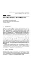
not exceed R. An example of a unit disk graph model of a wireless multihop net-
work and a nominal schedule are shown in Figure 16.1. In that figure, there is a link
between a pair of stations if and only if the circles of radius R/2 centered at the pair
of stations intersect, including being tangent. The slots assigned to the stations are
the numbers inside the brackets.
Regardless of the graph model utilized, if there is an edge between nodes u and v, then u is
a one-hop neighbor/neighbor of v and likewise v is a neighbor of u. The degree of a node
is the number of neighbors. The degree
␳
of a network is the maximum degree of the
nodes in the network. The distance-2 neighbors of a node include all of its one-hop neigh-
bors and the one-hop neighbors of its one-hop neighbors. The two-hop neighbors of a
node are those nodes that are distance-2 neighbors, but are not one-hop neighbors. The

unit subset of node u consists of u and its distance-2 neighbors. The distance-2 degree
D(u) of u is the number of distance-2 neighbors of u, and the distance-2 degree D of a net-
work, is the maximum distance-2 degree of the nodes in the network.
Relevant to broadcast scheduling is distance-2 coloring [22, 13] of a graph G = (V, E),
where the problem is to produce an assignment of colors C : V Ǟ 1, 2, . . . such that no
two nodes are assigned the same color if they are distance-2 neighbors. An optimal color-
ing is a coloring utilizing a minimum number of colors. A distance-2 coloring algorithm is
said to color nodes in a greedy fashion (i.e., greedily) if when coloring a node, the color
16.2 WHAT IS BROADCAST SCHEDULING? 349
Figure 16.1 Broadcast scheduling modeled by a unit disk graph.
assigned is the smallest number color that can be assigned without resulting in conflicts.
Here, the constraint number of a node is the number of different colors assigned to the
node’s distance-2 neighbors.
In the context of broadcast scheduling, determining a nominal schedule is directly ab-
stracted to distance-2 coloring, whereby slots that are assigned to stations are translated
into colors that are assigned to nodes. In this chapter, we will interchangeably use the
terms network and graph, station and node, and slot and color.
16.2.4 Varieties of Broadcast Scheduling Algorithms
There are two main varieties of broadcast scheduling algorithms—centralized and distrib-
uted.
Centralized Algorithms
Centralized algorithms are executed at a central site and the results are then transmitted to
the other stations in the network. This requires that the central site have complete informa-
tion about the network. This is a strong assumption that is not easy to justify for wireless
multihop networks with mobile stations. The study of centralized algorithms, however,
provides an excellent starting point for both the theory of broadcast scheduling and the de-
velopment of more practical algorithms. Further, for some stationary wireless networks, it
is reasonable to run a centralized algorithm at the net management center and then distrib-
ute schedules to stations.
In the centralized algorithm context, there are two types of algorithms corresponding to

how the input is provided:
1. Off-line algorithms. The network topology is provided to the central site in its en-
tirety. The algorithm computes the schedule for the entire network once and for all.
2. Adaptive algorithms: With off-line algorithms, if the network topology changes,
then the algorithm is rerun for the entire network. However, as wireless networks
are evolving towards thousands of stations spread over a broad geographical area
and operating in an unpredictable dynamic environment, the use of off-line schedul-
ing algorithms is not realistic. In practice, it is absolutely unaffordable to halt com-
munication whenever there is a change in the network, so as to produce a new
schedule “from scratch.” In such circumstances, adaptive algorithms are required
That is, given a broadcast schedule for the network, if the network changes (by the
joining or leaving of a station), then the schedule should be appropriately updated to
correspond to the modified network. Thus, an adaptive algorithm for broadcast
scheduling is one that, given a wireless multihop network, a broadcast schedule for
that network, and a change in the network (i.e., either a station joining or leaving the
network), produces a broadcast schedule for the new network. The twin objectives
of adaptive algorithms are much faster execution (than an off-line algorithm that
computes a completely new schedule) and the production of a provably high-quality
schedule. We note that many other network changes can be modeled by joining or
leaving or a combination of the two (e.g., the moving of a station from one location
to another).
350
BROADCAST SCHEDULING FOR TDMA IN WIRELESS MULTIHOP NETWORKS
Distributed Algorithms
Although centralized algorithms provide an excellent foundation, algorithms in which the
computation is distributed among the nodes of the network are essential for use in prac-
tice. In these distributed algorithms, network nodes have only local information and par-
ticipate in the computation by exchanging messages. Distributed algorithms are important
in order to respond quickly to changes in network topology. Further, the decentralization
results in decreased vulnerability to node failures. We distinguish between two kinds of

distributed algorithms:
1. Token passing algorithms. A token is passed around the network. When a station
holds the token, it computes its portion of the algorithm [26, 2]. There is no central
site, although a limited amount of global information about the network may be
passed with the token. Token passing algorithms, while distributing the computa-
tion, execute the algorithm in an essentially sequential fashion.
2. Fully distributed algorithms. No global information is required (other than the glob-
al slot synchronization associated with TDMA), either in individual or central sites.
Rather, a station executes the algorithm itself after collecting information from sta-
tions in its local vicinity. Multiple stations can simultaneously run the algorithm, as
long as they are not geographically too close, and stations in nonlocal portions of
the network can transmit normally even while other stations are joining or leaving
the network. Fully distributed algorithms are essentially parallel, and are typically
able to scale as the network expands.
16.3 THE COMPLEXITY OF BROADCAST SCHEDULING
In this section the computational complexity of broadcast scheduling is studied.
16.3.1 Computing Optimal Schedules
As noted in the previous section, determining a minimum nominal schedule in a wireless
multihop network is equivalent to finding a distance-2 graph coloring that uses a mini-
mum number of colors. The NP-completeness of distance-2 graph coloring is well estab-
lished [22, 6, 26, 5]. The strongest of these [6] shows that distance-2 graph coloring re-
mains NP-complete even if the question is whether or not four colors will suffice. They
utilize a reduction from standard graph coloring. Thus:
Theorem 1 Given an arbitrary graph and an integer k Ն 4, determining if there exists a
broadcast schedule of length not exceeding k, is NP-complete.
By way of contrast, in [25] it is shown that when k is three, the problem can be solved in
polynomial time. Given the NP-completeness of the basic problem, we are left with the
possible approaches of utilizing approximation algorithms to determine approximately
minimal solutions, or considering the complexity on restricted classes of graphs. Most of
the remainder of this chapter is devoted to the former. In regard to the latter, we note:

16.3 THE COMPLEXITY OF BROADCAST SCHEDULING 351
Theorem 2 [25] Given a planar graph, determining if there exists a broadcast schedule
of length not exceeding seven, is NP-complete.
16.3.2 What About Approximations?
From the NP-completeness results cited above, finding minimum length broadcast
schedules is generally not possible. Thus, it is necessarily the case that we focus on al-
gorithms that produce schedules that are approximately minimal. For such an approxi-
mation algorithm, its approximation ratio
␣
[8, 10], is the worst case ratio of the length
of a nominal schedule produced by the algorithm to the length of an optimal nominal
schedule. Such an algorithm is said to produce
␣
-approximate solutions. In the context
of adaptive algorithms, the analagous concept is that of a competitive ratio. Here, the ra-
tio is the length of the current nominal schedule produced by the algorithm to an opti-
mal off-line nominal schedule. Additional information on such ratios and alternatives
may be found in [8, 10].
What quality of approximation ratio might be possible for broadcast scheduling? Most
often, the goal in designing approximation algorithms is to seek an approximation ratio
that does not exceed a fixed constant (i.e., a constant ratio approximation algorithm). One
would hope, as in bin packing and geometric traveling salesperson [10], that approxima-
tion ratios of two or less might be possible. Unfortunately, this is not the case, not only for
any fixed constant, but also for much larger ratios:
Theorem 3 [1] Unless NP = ZPP, broadcast scheduling of arbitrary graphs cannot be
approximated to within O(n
1/2–
⑀
) for any
⑀

> 0.
This result is tight since there is an algorithm (see the next section) having an approxi-
mation ratio that is O(n
1/2
).
16.4 CENTRALIZED ALGORITHMS
Since broadcast scheduling is NP-complete, in this section (and the next) we investigate
approximation algorithms that are alternatives to producing optimal schedules. These al-
gorithms are evaluated on the basis of their running times and approximation ratios.
16.4.1 A Classification of Approximation Algorithms for
Broadcast Scheduling
An overview of approximation algorithms for broadcast scheduling is given in this sec-
tion. Only a few particular algorithms are specifically described, and the reader is referred
to [11, 25] for a more comprehensive treatment.
In developing approximation methods for broadcast scheduling, the classic algorithm
P_Greedy takes a purely greedy approach. That algorithm is an iterative method in which
a node is arbitrarily chosen from the as yet uncolored nodes and is greedily colored. The
running time of P_Greedy is O(n
␳
2
) on arbitrary graphs and O(n
␳
) on unit disk graphs.
352
BROADCAST SCHEDULING FOR TDMA IN WIRELESS MULTIHOP NETWORKS
The approximation ratio of P_Greedy is min(
␳
, n
1/2
) [26, 22] on arbitrary graphs, and 13

on unit disk graphs [18].
Aside from P_Greedy, a variety of centralized approximation algorithms have been
proposed for broadcast scheduling. These algorithms can be placed into three general cat-
egories, using a classification adapted from [11]:
1. Traditional algorithms that preorder the nodes according to a specified criterion,
and then color the nodes in a greedy fashion according to that ordering. A represen-
tative of such methods is Static_min_deg_last [11]. In this method, the nodes are
placed into descending order according to their degrees. The nodes are then greedi-
ly colored according to that ordering. The running time is O(n min(n,
␳
2
)) on arbi-
trary graphs and O(n log n + n
␳
) on unit disk graphs. The algorithm is
␳
-approxi-
mate on arbitrary graphs, and 13-approximate on unit disk graphs [18].
2. Geometric algorithms that involve projections of the network onto simpler geomet-
ric objects, such as the line. A representative of such methods is Linear_Projection
[11], in which the positions of the nodes are projected onto a line, and then an opti-
mal distance-2 coloring is computed for those projected points. One effect of pro-
jecting nodes onto a line is that the projections of nodes may now be within dis-
tance-2, whereas the original nodes were not within distance-2. The algorithm
selects a line for projection that minimizes the number of such “false” distance-2
neighbors. Linear_Projection runs in time O(n
2
) on arbitrary graphs. There are no
results on the approximation ratio.
3. Dynamic greedy methods that also color nodes in a greedy fashion, but in which the

order of the coloring is determined dynamically as the coloring proceeds. A repre-
sentative of such methods is max_cont_color [16]. This algorithm initially colors an
arbitrary node and then all of the one-hop neighbors of that node. At each subse-
quent step, the algorithm chooses for coloring a node that is now most constrained
by its distance-2 neighbors. Results [16, 18] show that this algorithm has the best
simulation performance among all existing broadcast scheduling algorithms. A
careful implementation [18] yields a running time of O(nD) on arbitrary graphs and
O(n
␳
) on unit disk graphs. The algorithm is
␳
-approximate on arbitrary graphs, and
13-approximate on unit disk graphs [18].
16.4.2 A Better Approximation Ratio
The best approximation ratio for arbitrary graphs of the methods cited above is
min(n
1/2
,
␳
), which is also the ratio of the simplest of these algorithms, P_Greedy. Below,
an algorithm of the “traditional greedy” variety is described that has an arguably stronger
ratio for most graphs. The algorithm is similar to Static_min_deg_last but the nodes are
ordered in a “dynamic,” rather than static, fashion. The term progressive is taken from [23].
Algorithm progressive_min_deg_last(G)
Labeler(G, n);
for j ǟ 1 to ndo
16.4 CENTRALIZED ALGORITHMS 353
let u be such that L(u) = j;
greedily color node u;
The function Labeler, which assigns a label between 1 and n to each node, is defined as

follows:
Labeler(G, ᐉ)
if G is not empty
let u be a vertex of G of minimum degree;
L(u) ǟ ᐉ;
Labeler(G – u, ᐉ – 1);
Here, G-u is the graph obtained from G by removing u and all incident edges. It is
straightforward to see that progressive_min_deg_last produces a legal coloring, since the
coloring is performed in a greedy fashion. This will be true for all of the algorithms de-
scribed in this chapter, and we will make no further reference to algorithm correctness.
Theorem 4 For a planar graph, progressive_min_deg_last is 9-approximate.
Proof: Consider the neighbors of an arbitrary node u, and suppose that k of those nodes
have labels smaller than L(u). Hence, there are up to
␳
– k neighbors of u with labels larg-
er than L(u).
It follows from the properties of planar graphs, and the specification of Labeler, that k
Յ 5. Each node with a label smaller than L(u) may have at most
␳
– 1 neighbors (not in-
cluding u) and hence those k nodes and their neighbors utilize at most k(
␳
– 1) + k = k
␳
colors that may not be assigned to u.
Now consider the up to
␳
– k nodes with labels larger than L(u). When u is colored,
none of these nodes are colored (recall that coloring is done in increasing order of labels).
However, the neighbors of these nodes may have lower labels than L(u) and the already as-

signed colors of these nodes may not be assigned to u. Since the minimum node degree in
a planar graph is always five or less, it follows from the specification of Labeler that there
can be at most 4 · (
␳
– k) 2-hop neighbors of u that are already colored (i.e., four for each
uncolored 1 – hop neighbor of u, not counting u itself).
Thus, u can be colored using no more than k
␳
+ 4·(
␳
– k) + 1 colors, and with k Յ 5,
this is at most 9
␳
– 19. Since the minimum coloring uses at least
␳
+ 1 colors, the approx-
imation ratio is bounded above by nine. Ǣ
For arbitrary graphs, the approximation ratio of progressive_min_deg_last depends on
the thickness of the graph. That is, the minimum number of planar graphs into which the
graph may be partitioned. Note that the algorithm does not compute the thickness (indeed,
computing the thickness is NP-complete [21]), but rather only the bound depends on that
value. Further, experimental results [25] establish that the thickness is generally much less
than
␳
.
Corollary 1 For an arbitrary graph of thickness
␪
, progressive_min_deg_last has an ap-
proximation ratio that is O(
␪

).
354
BROADCAST SCHEDULING FOR TDMA IN WIRELESS MULTIHOP NETWORKS
The corollary follows from the prior proof by noting that in a graph of thickness
␪
, there is
at least one node of degree not exceeding 6
␪
– 1 [25].
The analysis in [14] establishes:
Theorem 5 For q-inductive graphs, progressive_min_deg_last has an approximation ra-
tio of 2q – 1.
Several classes of graphs, including graphs of bounded genus, are q-inductive. See [12]
for additional information on q-inductive graphs.
In regard to running times, it is shown in [24]:
Theorem 6 For planar graphs, progressive_min_deg_last has a running time of O(n
␳
).
For arbitrary graphs of thickness
␪
, progressive_min_deg_last has a running time of
O(n
␪␳
).
16.4.3 A Better Ratio for Unit Disk Graphs
Among the methods cited above, several are 13-approximate when applied to unit disk
graphs. These ratios follow from a general result of [18] on the performance of “greedy”
algorithms. The best approximation ratio relative to unit disk graphs belongs to the follow-
ing algorithm (of the traditional greedy variety):
Algorithm Continuous_color(G):

Let u be an arbitrary node of G;
L
ǟ
a list of the nodes of G sorted in increasing order of Euclidean distance to u;
while L

0/ do
Let v be the first node of L;
Greedily color v and remove v from L;
Theorem 7 For unit disk graphs, Continuous_color has an approximation ratio of seven.
Key to the proof of this theorem is the following result that establishes that certain
nodes in geographical proximity to one another must be distance-2 neighbors.
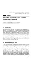
Lemma 1 Given a node p, let b
1
and b
2
be two points on the boundary of p’s interference
region (i.e., the circle of radius 2R centered at p). If |b
1
b
2
| Յ R, then any two nodes that are
both:
ț in the unit subset of p, and
ț within the area bounded by the line segments from p to b
1
and b
2
and by the bound-
ary of the interference region of p that runs between b

1
and b
2
(we refer to this area
as section pb
1
b
2
and show it as the shaded area in Figure 16.2)
are distance-2 neighbors.
16.4 CENTRALIZED ALGORITHMS 355
The proof of Lemma 1 involves the extensive use of trigonometric functions to establish
the proximity of points, and may be found in [18].
Proof: From Continuous_color, when a node v is to be colored, the already colored dis-
tance-2 neighbors of v lie on at most half of v’s interference region. The perimeter of that
half of an interference region can be partitioned into seven sections such that the distance
between the extreme perimeter points in each section does not exceed R. Within each of
these sections, from Lemma 1, all of the nodes are distance-2 neighbors, hence each of the
nodes must receive a distinct color. Let x be the largest number of nodes in any one of
these sections. Then x + 1 is a lower bound on the number of different colors assigned to v
and its already colored neighbors. Likewise, 7x + 1 is an upper bound on the number of
different colors used by Continuous_color. The theorem follows from the ratio of the up-
per to lower bound. Ǣ
In regard to running time, it is easy to see that the running time of Continuous_color is
O(n log n +nD) when applied to arbitrary graphs. Since D may be as large as
␳
2
, we have:
Lemma 2 For arbitrary graphs, the running time of Continuous_color is O(n log n +
n

␳
2
).
For unit disk graphs the running time is less. Key to that result is the following, which
establishes that D and
␳
are linearly related:
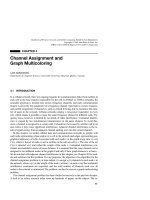
Lemma 3 In unit disk graphs, D Յ 25
␳
.
Proof: Consider the interference region of an arbitrary node s in a unit disk graph. Clear-
ly, all distance-2 neighbors of s lie within the interference region of s. Now, define an S-
cycle to be a circle of radius R/2 (it could be centered anywhere) and note that all nodes
lying within any given S-cycle are one-hop neighbors. Thus, at most
␳
nodes lie within any
given S-cycle. The lemma follows since the interference region of any node can be cov-
ered with 25 S-cycles as shown in Figure 16.3 (in that figure, S-cycles are shown both
shaded and unshaded to make them easier to visualize). Ǣ
356
BROADCAST SCHEDULING FOR TDMA IN WIRELESS MULTIHOP NETWORKS
Figure 16.2 The locations of b
1
and b
2
.
Corollary 2 For unit disk graphs, the running time of Continuous_color is O(n log n +
n
␳
).

16.4.4 An Adaptive Algorithm
An adaptive algorithm for broadcast scheduling is described in this section.
16.4.4.1 The Effects of the Joining and Leaving of Nodes
In designing adaptive algorithms, it is important to understand how the schedule might be
affected by the joining or leaving of a node (the algorithm presented in this section focus-
es on these basic functionalities):
ț The joining of a node may introduce conflicts among the node’s one-hop neighbors,
thus turning a previously conflict-free schedule into a conflicting schedule. An
adaptive broadcast scheduling algorithm must modify the existing schedule to re-
move these conflicts.
ț The leaving of a node never introduces conflicts into the schedule, though the
schedule may now be longer than necessary (though that is not easy to determine!).
Further, if A is the deleted node, that deletion may result in a neighbor of A with a
color larger than its number of distance-2 neighbors. The use of such a color is nev-
er required.
Algorithm_IR (Iteratively Remove) handles the joining of a node A as follows:
Algorithm IR_Station_Join(A)
increase the degree of the neighbors of A by 1;
update D(u) for each distance-2 neighbor u of A;
RECOLOR_LIST ǟ min_conflict_set(A);
16.4 CENTRALIZED ALGORITHMS 357
Figure 16.3 D Յ 25
␳
.
uncolor the nodes (if any) in RECOLOR_LIST;
add A to RECOLOR_LIST;
while RECOLOR_LIST  0/ do
v ǟ a node in RECOLOR_LIST with largest constraint number;
greedily color node v;
delete v from RECOLOR_LIST;

Within IR_Station_Join, function min_conflict_set(A) returns the minimum conflict set of
node A, determined as follows: Let U be the set consisting of all one-hop neighbors of A
that now conflict on a given color c (this occurs because the presence of A makes these
nodes into 2-hop neighbors). Among the nodes in U, let u
i
be a node with largest conflict
number. Then U – u
i
is a c-conflict clique of A. A minimum conflict set of A is the union
of its c-conflict cliques (one per color).
Algorithm_IR handles the leaving of a node as follows:
Algorithm IR_Station_Leave(A)
decrease the degree of the neighbors of A by 1;
update D(u) for each distance-2 neighbor u of A;
for each distance-2 neighbor u of Ado
if COLOR(u) > D(u) + 1
greedily recolor u;
We note that Algorithm_IR as given in [19, 18] contains a third procedure, maintenance.
That procedure, which attempts a recoloring around a node of maximum color after each
joining and leaving, is essential for the excellent performance of Algorithm_IR as mea-
sured by simulations. That additional procedure does not however affect (positively or
negatively) the approximation ratio, hence its omission from this chapter.
16.4.4.2 Approximation Ratio
To determine the approximation ratio of Algorithm_IR, we begin with the following lower
bound on the length of an optimal schedule:
Lemma 4 For unit disk graphs, an optimal schedule uses at least 1 + D/13 colors.
Proof: Recall that D is the distance-2 degree of the graph. Given a node v in a unit disk
graph, all of its distance-2 neighbors lie within the interference region of v. Partition the
interference region of v into 13 sections of equal angle around v. As in the proof of Theo-
rem 7, each section satisfies the conditions of Lemma 1, hence all of the distance-2 neigh-

bors of v within a given section are within distance-2 of one another. It follows that each
of the nodes in a given section must be assigned different colors. Thus, any coloring must
use at least 1 + D(v)/13 colors in coloring v and its distance-2 neighbors. Hence, an opti-
mal schedule for the graph uses at least 1 + D/13 colors. Ǣ
Theorem 8 For unit disk graphs, Algorithm_IR has an approximation ratio of 13.
358
BROADCAST SCHEDULING FOR TDMA IN WIRELESS MULTIHOP NETWORKS
Proof: For any unit disk graph consider the coloring produced by Algorithm_IR via a se-
quence of joinings and leavings of nodes. A careful consideration of IR_Station_Join and
IR_Station_Leave establishes the invariant that for each node v, COLOR(v) Յ 1 + D(v). It
follows that the algorithm uses at most 1 + D colors. Since by the prior lemma an optimal
schedule utilizes at least 1 + D/13 colors, the approximation ratio follows. Ǣ
An alternative algorithm with a 13-approximation ratio that handles the on-line joining
of stations appears in [27].
16.4.4.3 Running Time
An examination of the two procedures associated with Algorithm_IR shows that the run-
ning time for the joining or leaving of a node is bounded by O(
␳
2
+
␳
D + D
2
). How are
␳
and D related? Lemma 3 establishes that D is O(
␳
) in unit disk graphs, hence:
Theorem 9 For unit disk graphs, the worst case running time for the joining or leaving
of a node is O(

␳
2
). The time for an arbitrary graph is O(
␳
4
).
How good is this running time? For coloring a unit disk graph of n nodes the running
times of P_greedy and max_cont_color are both O(n
␳
), whereas the running time for Con-
tinuous_color is O(n log n + n
␳
). When applied in sequence to n nodes, Algorithm_IR
runs in time O(n
␳
2
), which is a loss of O(
␳
) in comparison with the centralized algorithms.
But that comparison is to a single execution of P_greedy or max_cont_color. In the ab-
sence of an adaptive algorithm, the only alternative when the graph changes is to recom-
pute the entire schedule, which requires time per change of O(n
␳
) using P_greedy or
max_cont_color. Since typically
␳
Ӷ n, the O(
␳
2
) time required by Algorithm_IR is much

superior for unit disk graphs.
16.5 DISTRIBUTED ALGORITHMS
Two distinctly different distributed algorithms are described in this section. The first uti-
lizes token passing to distribute the computation, and has a strong approximation ratio
when applied to arbitrary graphs. The second is a fully distributed algorithm based on
moving away from simply computing a nominal schedule, and has a constant approxima-
tion ratio when applied to unit disk graphs.
16.5.1 A Token Passing Algorithm
We begin by describing an efficient token passing algorithm for broadcast scheduling. A
first attempt would be to implement the progressive_min_deg_last algorithm using token
passing. However, the labeling phase of that algorithm requires that nodes be labeled in a
precise order, and it may be that consecutively numbered nodes are quite far apart in the
network. Reconciling this in a token-passing approach seems to be problematic.
In the algorithm described here, nodes are partitioned into classes based on the degrees
16.5 DISTRIBUTED ALGORITHMS 359
of the nodes. Coloring is then done in inverse order, starting with the last class. The nodes
of a class are colored in a single pass over the network.
16.5.1.1 The Algorithm DBS
For clarity, a centralized version of the algorithm is presented first. A discussion of a dis-
tributed implementation follows the algorithm.
The algorithm is parameterized, taking as input a parameter
␶
. Typically this parameter
would be fixed for a given network. There is a trade-off between
␶
and the number of pass-
es the algorithm makes over a network. This trade-off and explanations of the algorithm
will become apparent in the analyses of running time and approximation ratio that follow
the algorithm specification.
Algorithm DBS(G,

␶
)
classcnt ǟ 0;
neededratio ǟ (
␶
– 6)/
␶
;
incrementratio
ǟ
␶/6;
thickness ǟ 1;
currsize ǟ n;
The Assign Classes Phase:
while there exists a node v not yet assigned to a class do
classcnt++;
found ǟ 0;
for each node v not yet assigned to a class do
deglocal ǟ the number of 1-hop neighbors of v who were not yet in a class at the
start of this iteration of the while loop;
if deglocal Յ
␶
*thickness
assign v to class classcnt;
found++;
if found < currsize*neededratio
thickness ǟ incrementratio*thickness;
currsize ǟ currsize – found;
The Coloring Phase:
for i ǟ classcnt downto 1 do

for each node v in class ido
greedily color v;
16.5.1.2 The Running Time of DBS
A critical issue in limiting the running time of DBS, and the number of passes that it
makes over the network, is the number of classes into which the nodes are partitioned. The
following lemma [17] is helpful in that regard:
Lemma 5 Given an arbitrary graph G of thickness
␪
, and a parameter
␶
> 6, there are at
least (
␶
– 6)n/
␶
nodes of degree not exceeding
␶␪
.
360
BROADCAST SCHEDULING FOR TDMA IN WIRELESS MULTIHOP NETWORKS
It follows from this lemma that if graph G is of thickness
␪
and
␶
is 12, then at least one-
half of the nodes in G are of degree not exceeding 12
␪
. Thus, in the execution of DBS, the
first class will contain at least one half of the nodes in G, and the second class will contain
at least one quarter of the nodes in G, and so on. All together there will be no more than

log
2
n classes. More generally, it follows from Lemma 5 that:
Given an arbitrary graph G of thickness
␪
, and
␶
> 6, then the number of classes does not
exceed log
␶
/6
n.
Thus, it would seem that there is a range of suitable values for
␶
. Unfortunately, the above
results are based on knowing the thickness of the network and, as mentioned previously, it
is NP-complete to determine the thickness of an arbitrary network. Thus, we need a way of
estimating the thickness. Fortunately, a natural approach is suggested by Lemma 5. Name-
ly, given an estimate for the thickness, say
␪
e
, construct a class consisting of all of the
nodes of degree not exceeding
␶␪
e
. If the number of nodes in the class is at least (
␶
– 6)n/
␶
,

then all is well. If, on the other hand, the number of nodes is less than (
␶
– 6)n/
␶
, then the
current value of
␪
e
is less than the actual thickness, and the value of
␪
e
is increased before
forming the next class. The process continues in this fashion with: classes being formed;
the size of the class compared to the known bound; and, if the class is too small, then the
estimate of the thickness increased. The only care that needs to be taken is to not increase
the estimate too quickly (it would make classes very large and not spread nodes among
classes) or too slowly (there will be too many classes, hence too many passes over the net-
work will have been made). Fortunately, it is possible to increase the estimate of
␪
at an in-
termediate pace that is satisfactory from both points of view. These ideas form the basis of
the proof given in [17] that establishes:
Lemma 6 DBS makes O(log n) passes over the graph.
This lemma and a careful examination of DBS provides:
Lemma 7 For arbitrary graphs, the running time of DBS is O(n
␳
log n + n
␳
2
).

16.5.1.3 An Approximation Ratio for DBS
Theorem 10 For a graph of thickness
␪
, DBS has an approximation ratio of O(
␪
).
Recall from our earlier discussion that most previous broadcast scheduling algorithms
have an O(
␳
) bound on their performance. Since
␪
is generally much less than
␳
, the per-
formance of DBS may be markedly superior to that of earlier algorithms (depending on
the constants involved).
The proof of the theorem may be found in [17]. Here we consider only a key lemma:
Lemma 8 Let
␪
f
be the final value of thickness utilized by DBS, and let
␪
a
be the actual
thickness of the network G. Then,
␪
f
Յ (
␶
/6)␪

a
.
16.5 DISTRIBUTED ALGORITHMS 361
Proof: To establish the lemma, we show that in DBS, once the value of the variable thick-
ness is at least
␪
a
, the value of thickness will never again be modified. To see that is so,
consider any iteration of the while-loop after thickness has attained a value that is at least
that of
␪
a
. At that point in the algorithm, the only nodes that are of relevance are those that
have not yet been placed into some class. Thus, consider the graph restricted to those
nodes and the edges between them. Let
␪
Ј be the thickness of this reduced graph and note
that
␪
ЈՅ
␪
a
. It follows from results in [17] that there are at least currsize · neededratio
nodes of degree not exceeding
␶␪Ј
. But, since
␪
ЈՅ
␪
a

Յ
␪
f
, there are at least currsize ·
neededratio nodes of degree not exceeding
␶␪
a
. Thus, the value of found will be at least
currsize · neededratio, hence thickness will not be modified. Ǣ
16.5.1.4 A Token Passing Implementation
To implement DBS using token passing is straightforward. Recall that a token is passed
around the network and only the node holding the token can execute the algorithm. The
path taken by the token is a depth first search of the network. Then:
1. Each iteration of the while loop corresponds to a pass through the network.
2. The only pieces of global information required by a processor are: 1) an indication
of the phase that the algorithm is in (Assign Classes or Coloring), along with the
class number in that phase; 2) the current value of the variable thickness; and 3) a
count of the number of nodes that have been visited on this pass. These several
pieces of information can be passed along with the token itself.
3. Within each pass in the Assign Classes phase, when a node receives the token, if
that node has already been assigned to a class, it simply passes the token on. If the
node is not yet assigned to a class, then it is easy for that node to check on the num-
ber of its neighbors also not yet assigned to a class (as of the start of this iteration of
the while loop), and if appropriate, to assign itself to the current class.
4. Within each pass of the Coloring phase, a node colors itself by querying its dis-
tance-2 neighbors so as to determine their colors (if any).
16.5.2 A Fully Distributed Algorithm
A fully distributed algorithm for broadcast scheduling is presented in this section. The al-
gorithm is distinguished in the following ways:
ț It is assumed that stations have the capacity of global slot synchronization (i.e., stan-

dard TDMA).
ț No global information is required, either in central or individual sites. Rather, a sta-
tion schedules itself after collecting information from its one-hop and two-hop
neighbors.
ț The method is fully distributed. Thus, multiple stations can simultaneously run the
scheduler portion of the protocol, and stations in nonlocal portions of the network
can transmit normally even while other stations are joining or leaving the network.
ț The method has a constant competitive ratio (though admittedly large: 26).
362
BROADCAST SCHEDULING FOR TDMA IN WIRELESS MULTIHOP NETWORKS
This algorithm is termed Power of Two Scheduling (POTS) (named FDAS in [20]). There
are three aspects to the algorithm: the basic scheduling method, the adaptive implementa-
tion, and the distributed implementation. In the next three sections these are addressed in
turn.
16.5.2.1 Power of Two Scheduling
Diverging from the “nominal schedule” approach taken in earlier sections, we consider a
scheduling framework that focuses on determining two essential components for each sta-
tion: its transmission slot and its transmission cycle. A station transmits for the first time
in its transmission slot, and then every transmission cycle number of slots thereafter. Thus,
the transmission cycle is a fixed number of slots between two consecutive transmissions.
Interestingly, nominal schedules can also be framed in this context. In nominal sched-
ules, the transmission cycle is the same for each station, hence each station needs to know
not only which slot it is assigned, but also the maximum slot in the entire nominal schedule.
The approach taken in POTS is that a priori there is no reason why each station must
utilize the same transmission cycle as every other. For correctness,* all that is required is
that transmissions be received collision-free and that each station have a periodic opportu-
nity to transmit. Thus, POTS utilizes nonuniform transmission cycles. By so doing, each
station produces its transmission slot and transmission cycle locally, without the need for
global information.
Since the transmission slot specifies the first time that a station transmits, the assign-

ment of a transmission slot to a station is identical to the problem faced in algorithms us-
ing the nominal schedule approach. Specifically, a transmission slot must be assigned to a
station so as not to conflict with the transmission slots of the station’s distance-2 neigh-
bors. This is identical to distance-2 coloring, and the coloring terminology is utilized in
specifying the algorithm.
Algorithm POTS_Slot_Assign(A)
RECOLOR_LIST
ǟ
min_conflict_set(A);
uncolor the nodes in RECOLOR_LIST;
add A to RECOLOR_LIST;
while RECOLOR_LIST

0/ do
v ǟ a node in RECOLOR_LIST with largest constraint number;
T_SLOT(v) ǟ least color not used by v’s distance-2 neighbors;
delete v from RECOLOR_LIST;
Here, min_conflict_set(A) is as specified in Section 16.4.
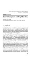
Now, suppose that all stations have been assigned transmission slots. Consider a station
u, and let C
u
denote the maximum transmission slot of any station in the unit subset of u.
Then, the transmission cycle for u is set to the least power of two that is greater than or
equal to C
u
. Figure 16.4 provides an example of a schedule derived from transmission
slots and cycles.
16.5 DISTRIBUTED ALGORITHMS 363
*On the issue of fairness (since some stations transmit more frequently than others), note that experimental re-
sults [18] show that relatively little is lost in overall schedule length when compared with nominal schedules.

364
BROADCAST SCHEDULING FOR TDMA IN WIRELESS MULTIHOP NETWORKS
Figure 16.4 Schedule derived using POTS.
In utilizing the transmission slot and cycle approach, the critical element is that there
are never any conflicts in the resulting schedule. The following theorem establishes that
this is indeed the case:
Theorem 11 For any two stations A and B that are distance-2 neighbors, if A and B are
assigned transmission slots and cycles as specified above, then A and B never transmit in
the same slot.
The proof follows in a straightforward fashion from a specification of the transmission
slots and cycles for A and B. The details appear in [20, 18].
16.5.2.2 Making the Method Adaptive
In this section, we describe how to extend the algorithm given above from the off-line to
the adaptive case.
The joining of stations is easy since an existing schedule can be updated to include the
joining station simply by running POTS_Slot_Assign (which may modify the transmission
slots of one-hop neighbors of the joining station) and then recomputing the transmission
cycle for each station in the unit subset of any station whose slot was modified. The only
additional issue is that some coordination is required to ensure that all stations, old and
new, are operating under an identical point of reference relative to the start of the sched-
ule. The details of this coordination are described in [18].
Since the leaving of a station from the network cannot introduce conflicts into the
schedule, the only scheduling effect produced by the leaving of a station is that the trans-
mission cycles of some of the stations may now be longer than necessary. Thus, when a
station leaves the network, some adjustments of the schedule may be appropriate. These
adjustments concern the transmission slot assignment of nodes in the unit subset of the
leaving station. The details are provided below.
Algorithm POTS_Deletion(A)
for each one-hop and two-hop neighbor u of Ado
update the degree of u and/or D(u) as appropriate;

if T_SLOT(u) > D(u) + 1
greedily recolor u;
for each node that had a member of its unit subset change color do
update the transmission cycle of that node;
16.5.2.3 The Approximation Ratio and Running Time
In the context of broadcast scheduling based on transmission slots and cycles, we define
the approximation ratio of an algorithm to be the ratio of the maximum transmission cycle
produced by the algorithm to the optimal maximum transmission cycle. In that context:
Theorem 12 For unit disk graphs, POTS has a competitive ratio of 26.
Proof: Using Lemma 1, it can be shown that the ratio of the maximum transmission slot to
the optimal maximum transmission cycle is bounded above by 13. Since the maximum
16.5 DISTRIBUTED ALGORITHMS 365
transmission cycle is less than twice the maximum transmission slot, the competitive ratio
of 26 follows. Ǣ
Finally, in regard to the running time of POTS:
Theorem 13 The running times of POTS_Slot_Assign and POTS_Deletion are O(
␳
2
) for
unit disk graphs [18], and O(
␳
4
) for arbitrary graphs.
Note that these match the running times of the adaptive Algorithm_IR of the previous
section.
16.5.2.4 Making the Method Fully Distributed
The key to producing a distributed implementation of POTS is to note that the scheduling
of a station requires NO global information. Rather, information is required only from the
one and two-hop neighbors of the station. In this respect, implementing the algorithm in a
distributed fashion is straightforward: from the perspective of an individual station, its ac-

tions in regard to scheduling precisely follow the method outlined above. The only com-
plications arise in the communication aspects, including: station registration when joining
the network, coordination of geographically close stations attempting to run the algorithm
in an overlapping fashion, and coordination of station actions when a neighboring station
leaves the network. Discussion of such an implementation is beyond the scope of this
chapter. The reader is referred to [18] for implementation details. An alternative fully dis-
tributed broadcast scheduling algorithm is given in [31].
16.6 RELATED RESULTS
This section provides an overview of some results related to broadcast scheduling.
16.6.1 Experimental Results
Almost all papers dealing with broadcast scheduling have included some experimental re-
sults. Most often these experiments have been conducted on networks that can be modeled
by unit disk graphs, although the networks are not often identified as such. The most com-
prehensive treatments to date are given in [11, 28], although the more recent algorithms of
[19, 20] are obviously not included there. In overall simulation performance, the algo-
rithm max_cont_color generally outperforms all others by at least a minimal amount. In
comparison [16] with P_Greedy, max_cont_color produces schedules (for unit disk
graphs) that are roughly 10% longer than optimal, while the schedules of P_Greedy aver-
aged nearly 30% longer than optimal. The algorithms Algorithm_IR and POTS likewise
outperform P_Greedy by a significant amount, although they are not as strong as
max_cont_color [18]. Due to its sometimes longer transmission cycles (due to being a
power of two), POTS is slightly weaker than Algorithm_IR. Finally, experimental results
detailing a gradual neural network broadcast scheduling algorithm are given in [7]. The
reader is referred to individual papers for specifics on experimental results for these and
many other algorithms.
366
BROADCAST SCHEDULING FOR TDMA IN WIRELESS MULTIHOP NETWORKS
16.6.2 Other Classes of Graphs
Aside from the results cited earlier in this chapter, only limited results are known for other
classes of graphs. Most notable among these are:

ț A proof that broadcast scheduling is NP-complete for intersection graphs of circles
is given in [28]. For these graphs, a 13-approximation algorithm is given in [27].
Unit disk graphs are a special type of intersection graph in which each circle has the
same radius.
ț A 2-approximation algorithm is given in [14] for (r, s )-civilized graphs [29]. Note
that (r, s )-civilized graphs include intersection (hence, unit disk) graphs provided
that there is a fixed minimum distance between the nodes. For these special types of
intersection and unit disk graphs, the 3-approximation of [14] is much superior to
the general bounds of 14 and 7, respectively.
ț For planar graphs, there is a 2-approximation algorithm [1].
ț For graphs whose treewidth is bounded by a constant k, optimal broadcast schedules
can be computed in polynomial time [30].
16.6.3 Link Scheduling
In the context of a wireless multihop network, link scheduling is an alternative to broad-
cast scheduling. In link scheduling, the links between the stations are scheduled such that
it is guaranteed that there will be no collision at the endpoints of the scheduled link, al-
though there may be collisions at nodes not scheduled to receive or transmit in that time
slot.
Analogous results to many of the broadcast scheduling results described in this chapter
have appeared for link scheduling. These include a pure greedy method, an algorithm with
an O(
␪
) approximation ratio for arbitrary graphs and an O(1) ratio for planar graphs, and
both token passing and fully distributed algorithms. Although the results are analogous to
those for broadcast scheduling, the methods, particularly those producing the O(
␪
) ap-
proximation ratios, are considerably more involved. The reader is referred to [25, 15, 4,
17, 24] for the details. A distributed link scheduling algorithm under somewhat different
assumptions is given in [4].

16.6.4 Unifying TDMA/CDMA/FDMA Scheduling
Frequency division multiplexing (FDMA) and code division multiplexing (CDMA) serve
as alternates to TDMA as channel access methods, although scheduling has been some-
what less studied in those contexts. In [23], an algorithm is given for scheduling regardless
of the channel access mechanism. That general algorithm is based on the
progressive_min_deg_last method described earlier.* The algorithm takes as input not
only a graph, but a general constraint set that specifies when nodes or links must receive
16.6 RELATED RESULTS 367
*In [23], the method is named progressive min degree first, with the “first” referring to the order in which nodes
are labeled.
different colors. It is shown in [23] that the algorithm has an approximation ratio of O(
␪
)
for any of some 128 problem variations.
16.7 SUMMARY AND OPEN PROBLEMS
This chapter studied the problem of broadcast scheduling in wireless multihop networks.
The focus was on complexity and algorithmic issues associated with such scheduling.
Since the basic problem is NP-complete, research has concentrated on the development of
approximation methods. In this chapter’s treatment of approximation algorithms, we have
attempted both to provide a flavor of the research issues and directions, and to enumerate
the strongest known results. Specifically:
ț For arbitrary graphs, there are centralized and token passing algorithms having O(
␪
)
approximation ratios. This is in comparison with the typical
␳
-approximations asso-
ciated with most other broadcast scheduling methods.
ț In unit disk graphs, the best centralized algorithm has an approximation ratio of sev-
en, while there is a fully distributed algorithm with a ratio of 26. The latter produces

schedules that allow stations to have different transmission cycles, thereby moving
away from the nominal schedule approach taken in other works.
In regard to open problems, we list only two general problems, and refer the reader to
individual research papers for more comprehensive lists.
ț From a theoretical perspective, there is tremendous room for improvement in all of
the approximation ratios. We do not believe that any of the cited ratios are tight.
ț From a practical perspective, the development and/or study of other graph models
appears important. None of the models studied to date appears to capture the situa-
tions that most often arise in practice. There, some concept of “almost” unit disk
graphs seems most appropriate in accounting for interference that eliminates some
links from the network.
ACKNOWLEDGMENTS
I would like to thank S.S. Ravi, Ram Ramanathan, and Xiaopeng Ma for providing com-
ments and suggestions on a draft version of this chapter.
REFERENCES
1. G. Agnarsson and M., Halldorsson. Coloring powers of planar graphs, Proceedings of the 11th
Annual Symposium on Discrete Mathematics (SODA), pp. 654–662, January 2000.
2. I. Chlamtac and S. Kutten, Tree-based broadcasting in multi-hop radio networks, IEEE Transac-
tions on Computers, 36: 1209–1223, 1987.
368
BROADCAST SCHEDULING FOR TDMA IN WIRELESS MULTIHOP NETWORKS
3. B. N. Clark, C. J. Colbourn, and D. S. Johnson, Unit disk graphs, Discrete Mathematics, 86:
165–167, 1990.
4. J. Flynn D. Baker, A., Ephremedes. The design and simulation of a mobile radio network with
distributed control, IEEE Journal on Selected Areas in Communications, SAC-2: 226–237,
1999.
5. A. Ephremedis and T. Truong, A distributed algorithm for efficient and interference free broad-
casting in radio networks, In Proceedings IEEE INFOCOM, 1988.
6. S. Even, O. Goldreich, S. Moran, and P. Tong, On the NP-completeness of certain network test-
ing problems, Networks, 14: 1–24, 1984.

7. N. Funabiki and J. Kitamichi, A gradual neural network algorithm for broadcast scheduling
problems in packet radio networks, IEICE Trans. Fundamentals, E82-A: 815–825, 1999.
8. M. R. Garey and D. S. Johnson, Computers and Intractability—A Guide to the Theory of NP-
Completeness, W. H. Freeman, San Francisco, 1979.
9. W. Hale, Frequency assignment: theory and applications, Proceedings of the IEEE, 68:
1497–1514, 1980.
10. D. S. Hochbaum, Approximation Algorithms for NP-hard problems, PWS, Boston, 1997.
11. M. L. Huson and A. Sen, Broadcast scheduling algorithms for radio networks, IEEE MILCOM,
pp. 647–651, 1995.
12. S. Irani, Coloring inductive graphs on-line, Algorithmica, 11: 53–72, 1994.
13. D. S. Johnson, The NP-completeness column, Journal of Algorithms, 3: 184, June 1982.
14. S. O. Krumke, M. V. Marathe, and S. S. Ravi, Models and approximation algorithms for channel
assignment in radio networks, Wireless Networks, 7, 6, 567–574, 2001.
15. R. Liu and E. L. Lloyd, A distributed protocol for adaptive link scheduling in ad-hoc networks,
in Proceedings of the IASTED International Conference on Wireless and Optical Communica-
tions, June 2001, pp. 43–48.
16. E. L. Lloyd and X. Ma, Experimental results on broadcast scheduling in radio networks,
Proceedings of Advanced Telecommunications/Information Distribution Research Program
(ATIRP) Conference, pp. 325–329, 1997.
17. E. L. Lloyd and S. Ramanathan, Efficient distributed algorithms for channel assignment in mul-
ti-hop radio networks, Journal of High Speed Networks, 2: 405–423, 1993.
18. X. Ma, Broadcast Scheduling in Multi-hop Packet Radio Networks. 2000. PhD Dissertation,
University of Delaware.
19. X. Ma and E. Lloyd, An incremental algorithm for broadcast scheduling in packet radio net-
works, in Proceedings IEEE MILCOM ‘98, 1998.
20. X. Ma and E. L. Lloyd, A distributed protocol for adaptive broadcast scheduling in packet radio
networks, in Workshop Record of the 2nd International Workshop on Discrete Algorithms and
Methods for Mobile Computing and Communications (DIAL M for Mobility), October 1998.
21. A. Mansfield, Determining the thickness of graphs is NP-hard, Math. Proc. Cambridge Philos.
Society, 93: 9–23, 1983.

22. S. T. McCormick, Optimal approximation of sparse Hessians and its equivalence to a graph col-
oring problem, Mathematics Programming, 26(2): 153–171, 1983.
23. S. Ramanathan, A unified framework and algorithm for channel assignment in wireless net-
works, Wireless Networks, 5: 81–94, 1999.
24. S. Ramanathan and E. L. Lloyd, Scheduling algorithms for multi-hop radio networks, IEEE/
ACM Transactions on Networking, 1: 166–177, 1993.
REFERENCES 369
25. S. Ramanathan, Scheduling Algorithms for Multi-hop Radio Networks, 1992. PhD Dissertation,
University of Delaware.
26. R. Ramaswami and K. K. Parhi, Distributed scheduling of broadcasts in a radio network, in
Proceedings IEEE INFOCOM, 1989.
27. A. Sen and E. Malesinska, On approximation algorithms for radio network scheduling, in Pro-
ceedings of the 35th Annual Allerton Conference on Communications, Control and Computing,
pp. 573–582, 1997.
28. A. Sen and M. L. Huson, A new model for scheduling packet radio networks, Wireless Net-
works, 3: 71–82, 1997.
29. S. H. Teng, Points, Spheres and Separators, A Unified Geometric Approach to Graph Separa-
tors, PhD Dissertation, Carnegie Mellon University, 1991.
30. X. Zhou, Y. Kanari and T. Nishizeki, Generalized vertex colorings of partial k-trees, IEICE
Transaction Fundamentals, E-A4: 1–8, 2000.
31. C. Zhu and M. S. Corson, A five-phase reservation protocol (FPRP) for mobile ad hoc net-
works, in Proceedings IEEE INFOCOM, pp. 322–331, 1998.
370
BROADCAST SCHEDULING FOR TDMA IN WIRELESS MULTIHOP NETWORKS