Tài liệu Sổ tay của các mạng không dây và điện toán di động P20 doc

CHAPTER 20
Dominating-Set-Based Routing
in Ad Hoc Wireless Networks
JIE WU
Department of Computer Science and Engineering, Florida Atlantic University
20.1 INTRODUCTION
An ad hoc wireless network is a special type of wireless network in which a collection of
mobile hosts with appropriate interfaces may form a temporary network, without the aid
of any established infrastructure or centralized administration. Communication in an ad
hoc wireless network is based on multiple hops. Packets are relayed by intermediate hosts
between the source and the destination; that is, routes between two hosts may consist of
hops through other hosts in the network. Mobility of hosts can cause unpredictable topol-
ogy changes. Therefore, the task of finding and maintaining routes in an ad hoc wireless
network is nontrivial.
We can use a simple graph G = (V, E) to represent an ad hoc wireless network, where V
represents a set of wireless mobile hosts and E represents a set of edges. An edge between
host pairs (v, u) indicates that both hosts v and u are within their wireless transmitter
ranges. Unless otherwise specified, we assume that all mobile hosts are homogeneous,
i.e., their wireless transmitter ranges are the same. In other words, if there is an edge e =
(v, u) in E, it indicates that u is within v’s range and v is within u’s range. Thus, the corre-
sponding graph is an undirected graph called a unit graph, in which connections of hosts
are determined by their geographical distances.
Routing in ad hoc wireless networks poses special challenges. In general, the main
characteristics of mobile computing are low bandwidth, mobility, and low power. Wireless
networks deliver lower bandwidth than wired networks and, hence, information collection
(during the formation of a routing table) is expensive. Mobility of hosts, which causes
topological changes of the underlying network, also increases the volatility of network in-
formation. In addition, the limitation of power leads users to disconnect mobile hosts fre-
quently in order to save power consumption. This feature may also introduce more failures
into mobile networks.
Traditional routing protocols in wired networks, which generally use either link state

[21, 23] or distance vectors [15, 22], are not suitable for ad hoc wireless networks. In an
environment with mobile hosts as routers, convergence to new, stable routes after dynamic
changes in network topology may be slow; this process could be expensive due to low
425
Handbook of Wireless Networks and Mobile Computing, Edited by Ivan Stojmenovic´
Copyright © 2002 John Wiley & Sons, Inc.
ISBNs: 0-471-41902-8 (Paper); 0-471-22456-1 (Electronic)
bandwidth. Routing information has to be localized to adapt quickly to changes such as
host movement. Cluster-based routing [19] is a convenient method for routing in ad hoc
wireless networks. In an ad hoc wireless network, hosts in a vicinity (i.e., physically close
to each other) form a cluster or clique, which is a complete subgraph. Each cluster has one
or more gateway hosts to connect to other clusters in the network. Gateway hosts (from
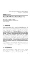
different clusters) are usually connected. In Figure 20.1, hosts u, v, and y form one cluster
and hosts w and x form another; v and w are gateway hosts which are connected. Back-
bone-based routing [6] and spine-based routing [7] use a similar approach. The backbone
(spine) consists of hosts similar to gateway hosts.
Note that gateway hosts form a dominating set [14] of the corresponding wireless net-
work. A subset of the vertices of a graph is a dominating set if every vertex not in the sub-
set is adjacent to at least one vertex in the subset. Moreover, this dominating set should be
connected for ease of routing within the induced graph consisting of dominating nodes
only. We refer to all routing approaches that use gateway hosts to form a dominating set as
dominating-set-based routing. The main advantage of dominating-set-based routing is that
it simplifies the routing process to one in a smaller subnetwork generated from the con-
nected dominating set. This means that only gateway hosts need to keep routing informa-
tion. As long as changes in network topology do not affect this subnetwork, there is no
need to recalculate routing tables.
Clearly, the efficiency of this approach depends largely on the process of finding and
maintaining a connected dominating set and the size of the corresponding subnetwork.
Unfortunately, finding a minimum connected dominating set is NP-complete for most
graphs. In this chapter, we consider a simple and efficient distributed algorithm that can

quickly determine a connected dominating set in ad hoc wireless networks. This algo-
rithm is a localized algorithm [11], hosts interact with others in a restricted vicinity.
Each host performs exceedingly simple tasks such as maintaining and propagating in-
formation markers. Collectively, these hosts achieve a desired global objective, i.e., find-
426
DOMINATING-SET-BASED ROUTING IN AD HOC WIRELESS NETWORKS
gateway host
u
y
non-gateway host
v
w
x
Figure 20.1 A sample ad hoc wireless network.
ing a small connected dominating set. It has been shown in [36] that this approach out-
performs several classical approaches in terms of finding a small dominating set and
does so quickly.
This chapter is organized as follows. Section 20.2 overviews the dominating set con-
cept, dominating-set-based routing, and related work. Section 20.3 discusses the decen-
tralized formation of a connected dominating set. Section 20.4 considers several exten-
sions, including networks with unidirectional links, hierarchical dominating sets,
power-aware routing, and multicasting and broadcasting. In Section 20.5 we summarize
the results and discuss future research in this area. Throughout the chapter, the terms
hosts, nodes, and vertices are used interchangeably.
20.2 PRELIMINARIES
20.2.1 Dominating Set
In the past quarter century, graph theory has experienced explosive growth concurrent
with the growth of computer science. One of the fastest-growing areas within graph theo-
ry is the study of domination and its related problems. Basically, a subset of the vertex set
in a graph is called a dominating set if every vertex in the graph is in the subset or is adja-

cent to an element of the subset.
The origin of the dominating set concept can trace back to the 1850’s, when the follow-
ing problem was considered among chess enthusiasts in Europe: Determine the minimum
number of queens that can be placed on a chessboard so that all squares are either attacked
by a queen or are occupied by a queen. It was found that five is the minimum number of
queens that can dominate all of the squares of an 8 × 8 chessboard. The five queen prob-
lem is about the placement of these five queens.
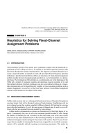
A real-life example of the dominating set concept is defining a school bus route within
a school district (see Figure 20.2). In this figure, black nodes are dominating nodes (also
called gateway nodes), and white nodes are dominated nodes (also called nongateway
20.2 PRELIMINARIES 427
gateway
non-gateway
school
0.5 mile
Figure 20.2 School bus route.
nodes). A bus route is defined based on certain rules. One such rule is that no student shall
have to walk farther than, say, half a mile to a bus pickup point. In addition, the route is
(strongly) connected. It is desirable that the length of the route be as short as possible.
Other applications of dominating sets include radio stations, social network theory, and
land surveying [14].
The domination number
␥
for a given graph is the size of the minimum dominating set.
Finding the domination number for a given graph is an NP-complete problem. Therefore,
most research in the graph theory community focuses on bounds on the domination num-
ber. Another area of focus is to determine special classes of graphs for which the domina-
tion problem can be solved in polynomial time.
20.2.2 Dominating-Set-Based Routing
Assume that a connected dominated set has been determined for a given ad hoc wireless

network. The routing process in dominating-set-based routing is usually divided into three
steps:
1. If the source is not a gateway host, it forwards the packets to a source gateway,
which is one of the adjacent gateway hosts.
2. This source gateway acts as a new source to route the packets in the induced graph
generated from the connected dominating set.
3. Eventually, the packets reach a destination gateway, which is either the destination
host itself or a gateway of the destination host. In the latter case, the destination
gateway forwards the packets directly to the destination host.
There are in general two ways to perform routing within the induced graph: proactive
routing and reactive routing. In proactive routing, routes to all destinations are computed a
priori and are maintained in the background via a periodic update process. In reactive
routing, a route to a specific destination is computed “on demand,” i.e., only when needed.
In the following, we use the destination-sequenced distance vector routing protocol
(DSDV) [26] as a sample proactive routing to illustrate the idea. It is critical to note that
routing within the induced graph is not limited to proactive routing, which usually uses
routing tables; reactive routing can also be applied. DSDV is based on the distributed Bell-
man–Ford (DBF) routing mechanism to construct routing tables. DBF is augmented with
sequence numbers so that mobile hosts can distinguish stale routes from new ones, there-
by avoiding the formation of routing loops.
Each nongateway host keeps an adjacent gateway list, whereas each gateway host keeps
the gateway domain member list and gateway routing table. The gateway domain member
list is a list of nongateway hosts that are adjacent to gateway hosts. The gateway routing
table includes one entry for each gateway host, together with its domain member list. For
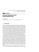
example, given an ad hoc wireless network as shown in Figure 20.3 (a), the corresponding
routing information at host 8 is shown in Figure 20.3 (b), which shows that host 8 has
three members—3, 10, and 11—in its gateway domain member list. Figure 20.3 (c) shows
the gateway routing table at host 8, which consists of a set of entries for each gateway and
428
DOMINATING-SET-BASED ROUTING IN AD HOC WIRELESS NETWORKS

its member list. The third column of this table shows the next-hop information of a short-
est path (here defined as a path with a minimum hop count) and the fourth column the dis-
tance (in hop count) to each destination.
20.2.3 Related Work
Routing protocols for wired networks can be classified into link state and distance vector
schemes. The link state approach [21] runs the centralized version of a shortest path algo-
rithm such as Dijkstra’s algorithm. The distance vector approach uses the distributed Bell-
man–Ford (DBF) algorithm [18]. Both approaches are not suitable for dynamic networks,
especially for quick-changing wireless networks such as ad hoc wireless networks. The
main problems are computational burden, bandwidth overhead, and slow convergence of
routing information. As indicated in [16, 26], these problems are especially pronounced in
ad hoc wireless networks that have low power, limited bandwidth, and unrestricted mobil-
ity.
Various design choices are available for designing routing protocols for ad hoc wireless
networks, they are:
20.2 PRELIMINARIES 429
9 (1,2,3,11)
4 (5,6)
7
(6)
9
7
7
1
2
1
3
10
11
(a)

gateway domain member list gateway routing table
destination member list next hop distance
(c)(b)
2
1
11
10
7
8
5
9
4
6
3
Figure 20.3 (a) A routing example. (b) Gateway domain member list of node 8. (c) Gateway rout-
ing table of node 8.
1. Proactive versus reactive
2. Flat versus hierarchical
3. GPS-based versus non-GPS-based
Other classifications of routing protocols can be found in [29]. In a flat routing
scheme, all hosts are treated equally and, therefore, any host can be used to forward pack-
ets between arbitrary sources and destinations. In general, a set of homogeneous processes
is applied at each host. These processes include information collection, mobility manage-
ment, and routing. To permit scaling, hierarchical techniques are usually applied. The ma-
jor advantage of hierarchical routing is the reduction of routing table storage and process-
ing (including searching) overhead [31, 33]. In non-GPS-based routing, the routing
process is based solely on the connections of hosts in the network. In GPS-based routing,
each host knows its physical location through geolocation techniques such as GPS. Rout-
ing is governed by physical location of the destination, that is, the packets are forwarded
toward the destination based on the physical location of the destination.

Among hierarchical routing schemes, the cluster-based algorithm [19] divides a given
graph into a number of nonredundant clusters that may overlap with each other. This ap-
proach can be considered as a restricted version of the dominating-set-based approach.
Each cluster is a clique that is a complete subgraph. A cluster is nonredundant if it cannot
be covered by a set of other clusters. One or more representative nodes, called boundary
nodes, is selected from each cluster to form a connected subnetwork in which the routing
process proceeds and this subnetwork forms a connected dominating set. Each boundary
node has a complete view of the subnetwork captured by an associated routing table. In
this way, the routing process reduces the whole network to a small connected subnetwork.
The routing protocol is completed in two phases: cluster formation and cluster mainte-
nance. Note that the initial cluster formation algorithm is fully sequential, causing a high
computational complexity. The resultant cluster structure also depends on the order in
which mobile hosts are examined in calculation. Lin and Gerla [20] proposed an efficient
distributed algorithm for clustering. However, it is rather complex to maintain the cluster
structure during host movement.
Das et al. [6, 7, 30] proposed a series of hierarchical routing algorithms for ad hoc
wireless networks. Similar to cluster-based routing, the idea is to identify a subnetwork
that forms a minimum connected dominating set (MCDS). Again, each node in the sub-
network maintains a routing table that captures the topological structure of the whole net-
work. Each node in the subnetwork is called a spine node or backbone node (or gateway
host in the dominating-set-based approach). The formation of MCDS is based on Guha
and Khuller’s approximation algorithm [13]. This MCDS calculation algorithm has sever-
al advantages over to the cluster-based approach [19]. The main drawback of this algo-
rithm is that it still needs a nonconstant number of rounds to determine a connected domi-
nating set. Other hierarchical routing protocols [4] exist that do not require cluster heads
(dominating nodes) to be connected. However, a different mobility management method is
used.
Johnson’s [17] dynamic source routing (DSR) is a reactive approach without construct-
430
DOMINATING-SET-BASED ROUTING IN AD HOC WIRELESS NETWORKS

ing the routing tables usually used in a proactive approach such as DSDV. Normally, the
resultant routing path is not the shortest. However, this protocol adapts quickly to route
changes when host movement is frequent, yet requires little or no overhead during periods
in which hosts move less frequently. The approach consists of route discovery and route
maintenance. Route discovery allows any host to dynamically discover a route to a desti-
nation host. Each host also maintains a route cache in which it caches source routes that it
has learned. Unlike regular routing-table-based approaches that have to perform periodic
route updates, route maintenance only monitors the routing process and informs the
sender of any routing errors. One can easily apply Johnson’s approach to dominating-set-
based routing, in which route discovery is restricted to the subnetwork containing the con-
nected dominating set.
Zone-based routing [25] is a compromise approach between proactive and reactive ap-
proaches. Each routing table keeps information for destinations within a certain distance
(the corresponding area is called a zone). Information for destinations outside the zone
area is obtained on an on-demand basis, i.e., through a route recovery phase as in DSR.
Also, zone-based routing limits topology update propagation to the neighborhood of the
change.
20.3 FORMATION OF A CONNECTED DOMINATING SET
As mentioned earlier, we focus on the decentralized formation of a dominating set. Some
desirable features for such a process are listed below:
ț The formation process should be distributed and simple. Ideally, it requires only lo-
cal information and a constant number of iterative rounds of message exchanges
among neighboring hosts.
ț The resultant dominating set should be connected and close to minimum.
ț The resultant dominating set should include all intermediate nodes of any shortest
path. In this case, an all-pair shortest paths algorithm only needs to be applied to the
subnetwork generated from the dominating set.
20.3.1 Marking Process
The marking process is a localized algorithm [11] in which hosts only interact with others
in a restricted vicinity. Each host performs exceedingly simple tasks such as maintaining

and propagating information markers. Collectively, these hosts achieve a desired global
objective, i.e., finding a small connected dominating set. The marking process marks
every vertex in a given connected and simple graph G = (V, E). m(v) is a marker for vertex
v ʦ V, which is either T (marked) or F (unmarked). We will show later that marked ver-
tices form a connected dominating set. We assume that all vertices are unmarked initially.
N(v) = {u|(v, u) ʦ E} represents the open neighbor set of vertex v. Initially, each vertex v
has its open neighbor set N(v).
20.3 FORMATION OF A CONNECTED DOMINATING SET 431
The Marking Process
1. Initially, assign marker F to each v in V.
2. Each v exchanges its open neighbor set N(v) with all its neighbors’.
3. Each v assigns its marker m(v) to T if there exist two unconnected neighbors.
In the example of Figure 20.1, N(u) = {v, y}, N(v) = {u, w, y}, N(w) = {v, x}, N(y) = {u,
v}, and N(x) = {w}. After Step 2 of the marking process, vertex u has N(v) and N(y), B has
N(u), N(w), and N(y), w has N(v) and N(x), y has N(u) and N(v), and x has N(w). Based on
Step 3, only vertices v and w are marked T.
Clearly, each vertex knows distance-2 neighborhood information after Step 2 of the
marking process, i.e., neighbor information of its neighbors. The cost of checking the con-
nectivity of two neighbors is upper bounded by ⌬
2
(G) or simply ⌬
2
, where ⌬ is the degree
of graph G, i.e., ⌬(G) = max{|N(v)||v ʦ V}. There are |N(v)|(|N(v)| – 1)/2 possible pairs of
neighbors of vertex v, which is upper bounded by ⌬
2
. Therefore, the cost of the marking
process at each vertex is O(⌬
2
). The amount of message exchange at each vertex is also

O(⌬), which corresponds to the number of neighbors.
20.3.2 Properties
Assume that VЈ is the set of vertices that are marked T in V, i.e., VЈ = {v|v ʦ V, m(v) = T}.
The induced graph GЈ is the subgraph of G induced by VЈ, i.e., GЈ = G[VЈ]. The following
two theorems show that GЈ is a connected dominating set of G.
Theorem 1 Given a graph G = (V, E) that is connected but not completely connected,
the vertex subset VЈ, derived from the marking process, forms a dominating set of G.
Proof: Randomly select a vertex v in G. We show that v is either in VЈ (a set of vertices in
V that are marked T) or adjacent to a vertex in VЈ. Assume that v is marked F. If there is at
least one neighbor marked T, the theorem is proved. If all its neighbors are marked F, we
consider the following two cases.
Case 1: All the other vertices in G are neighbors of v. Based on the marking process
and the fact that m(v) = F, all these neighbors must be pairwise connected, i.e., G is com-
pletely connected. This contradicts the assumption that G is not completely connected.
Case 2: There is at least one vertex u in G that is not adjacent to vertex v. Construct a
shortest path path, (v, v
1
, v
2
, , u), connecting vertices v and u. Such a path always ex-
ists since G is a connected graph. Note that v
2
is u when v and u are distance-2 apart in G,
i.e., d
G
(v, u) = 2. Also, v and v
2
are disconnected; otherwise, (v, v
2
, , u) is a shorter

path connecting v and u. Based on the marking process, vertex v
1
, with both v and v
2
as its
neighbors, must be marked T. Again this contradicts the assumption that neighbors of v
are all marked F. २
When the given graph G is completely connected, all vertices are marked F. This is
desirable, because if all vertices are directly connected, there is no need for gateway
hosts.
432
DOMINATING-SET-BASED ROUTING IN AD HOC WIRELESS NETWORKS
Theorem 2 The induced graph GЈ = G[VЈ] is a connected graph.
Proof: We prove this theorem by contradiction. Assume that GЈ is disconnected and v and
u are two disconnected vertices in GЈ. Assume dis
G
(v, u) = k + 1 > 1 and (v, v
1
, v
2
, , v
k
,
u) is a shortest path between vertices v and u in G. Clearly, all v
1
, v
2
, , v
k
are distinct;

and among them there is at least one v
i
such that m(v
i
) = F (otherwise, v and u are con-
nected in GЈ). On the other hand, the two adjacent vertices of v
i
, v
i–1
and v
i+1
, are not con-
nected in G; otherwise, (v, v
1
, v
2
, , v
k
, u) is not a shortest path. Therefore, m(v
i
) = T
based on the marking process. This brings a contradiction. २
The next theorem shows that, except for source and destination vertices, all intermedi-
ate vertices in a shortest path are contained in the dominating set derived from the mark-
ing process.
Theorem 3 The shortest path between any two nodes does not include any nongateway
node as an intermediate node.
Proof: We prove this theorem also by contradiction. Assume that a shortest path between
two vertices v and u includes a nongateway node v
i

as an intermediate node; in other
words, this path can be represented as (v, , v
i–1
, v
i
, v
i+1
, , u). We label the vertex
that precedes v
i
on the path as v
i–1
; similarly, the vertex that follows v
i
on the path is la-
beled as v
i+1
. Because vertex v
i
is a nongateway node, i.e., m(v
i
) = F, there must be a con-
nection between v
i–1
and v
i+1
. Therefore, a shorter path between v and u can be found as
(v, , v
i–1
, v

i+1
, , u). This contradicts the original assumption. २
Since the problem of determining a minimum connected dominating set of a given con-
nected graph is NP-complete, the connected dominating set derived from the marking
process is normally nonminimum. In some cases, the resultant dominating set is trivial,
i.e., VЈ = V or VЈ = { }. For example, any vertex-symmetric graph will generate a trivial
dominating set using the proposed marking process. However, the marking process is effi-
cient for an ad hoc wireless network where the corresponding graph tends to form a set of
localized clusters (or cliques). The simulation results shown in [36] confirm this observa-
tion. When the transmission radius of a mobile host is not too large, the proposed algo-
rithm generates a small connected dominating set.
20.3.3 Dominating Set Reduction
In the following, we propose two rules to reduce the size of a connected dominating set
generated from the marking process. We first assign a distinct ID, id(v), to each vertex v in
GЈ. N[v] = N(v) ʜ {v} is the closed neighbor set of v, as opposed to the open one, N(v).
Rule 1: Consider two vertices v and u in GЈ. If N[v] ʕ N[u] in G and id(v) < id(u), change
the marker of v to F if node v is marked, i.e., GЈ is changed to GЈ – {v}.
The above rule indicates that the closed neighbor set of v is covered by that of u and
20.3 FORMATION OF A CONNECTED DOMINATING SET 433
vertex v can be removed from GЈ if the ID of v is smaller than that of u. Note that if v is
marked and its closed neighbor set is covered by the one of u, it implies vertex u is also
marked. When v and u have the same closed neighbor set, the vertex with the smaller ID is
removed. It is easy to prove that GЈ – {v} is still a connected dominating set of G. The
condition N[v] ʕ N[u] implies that v and u are connected in GЈ.
In Figure 20.4 (a), since N[v] Ͻ N[u], vertex v is removed from GЈ if id(v) < id(u) and
vertex u is the only dominating node in the graph. In Figure 20.4 (b), since N[v] = N[u],
either v or u can be removed from GЈ. To ensure one and only one is removed, we pick the
one with the smaller ID.
Rule 2: Assume that u and w are two marked neighbors of marked vertex v in GЈ. If N(v)
ʕ N(u) ʜ N(w) in G and id(v) = min{id(v), id(u), id(w)}, then change the marker of v to

F.
The above rule indicates that when the open neighbor set of v is covered by the open
neighbor sets of two of its marked neighbors, u and w, if v has the smallest ID of the three,
it can be removed from GЈ. The condition N(v) ʕ N(u) ʜ N(w) in Rule 2 implies that u
and w are connected. The subtle difference between Rule 1 and Rule 2 is the use of open
and closed neighbor sets. Again, it is easy to prove that GЈ – {v} is still a connected domi-
nating set. Both u and w are marked, because the facts that v is marked and N(v) ʕ N(u) ʜ
N(w) in G usually do not imply that u and w are marked. Therefore, if one set of u and w is
not marked, v cannot be unmarked (change the marker to F). To apply Rule 2, an addition-
al step last step needs to be included in the marking process: If v is marked [m(v) = T],
send its status to all its neighbors.
Consider the example in Figure 20.4 (c). Clearly, N(v) ʕ N(u) ʜ N(w). If id(v) =
min{id(v), id(u), id(w)}, vertex v can be removed from GЈ based on Rule 2. If id(u) =
min{id(v), id(u), id(w)}, then vertex u can be removed based on Rule 1, since N[u] ʕ
N[v]. If id(w) = min{id(v), id(u), id(w)}, no vertex can be removed. Therefore, the ID as-
signment also decides the final outcome of the dominating set. Note that Rule 2 can be
easily extended to a more general case where the open neighbor set of vertex v is covered
by the union of open neighbor sets of more than two neighbors of v in GЈ. However, the
connectivity requirement for these neighbors is more difficult to specify at vertex v.
The role of ID is very important for avoiding “illegal simultaneous” removal of vertices
434
DOMINATING-SET-BASED ROUTING IN AD HOC WIRELESS NETWORKS
uvw
vu vu
(a) (b) (c)
Figure 20.4 Three examples of dominating set reduction.
in GЈ. In general, vertex v cannot be removed even if N[v] Ͻ N[u], unless id(v) < id(u).
Consider the example of Figure 20.4 (c) with id(v) = min{id(v), id(u), id(w)}. If the above
rule were not followed, vertex u would be unmarked to F (because N[u] ʚ N[v] even
though id(v) < id(u)); and based on Rule 2, vertex v would be unmarked to F. Clearly, the

only vertex w in VЈ does not form a dominating set any more.
20.3.4 Example
Figure 20.5 shows an example of using the proposed marking process and its extensions to
identify a set of connected dominating nodes. Each node keeps a list of its neighbors and
sends the list to all its neighbors. By doing so, each node has distance-2 neighborhood in-
formation, i.e., information about its neighbors and the neighbors of all its neighbors.
Node 1 does not mark itself as a gateway node because its only neighbors, 2 and 3, are
connected. Node 3 marks itself as a gateway node because there is no connection between
neighbors 1 and 4 (2 and 4). After node 3 marks itself, it sends its status to its neighbors 1,
20.3 FORMATION OF A CONNECTED DOMINATING SET 435
(a)
2
3
4
5
6
7
12
9
10
11
16
15
13
20
19
8
14
18
17

1
Figure 20.5 (a) Marked gateways without applying rules. (b) Marked gateways by applying Rules
1 and 2.
2
3
4
5
6
7
12
9
10
11
16
15
13
20
19
8
14
18
17
1
(b)
2, and 4. This gateway status is used to apply Rule 2 to unmark some gateway nodes to
nongateway nodes. Figure 20.5 (a) shows the gateway nodes (nodes with double cycles)
derived by the marking process without applying two rules.
After applying Rule 1, node 17 is unmarked to the nongateway status. The closed
neighbor set of node 17 is N[17] = {17, 18, 19, 20}, and the closed neighbor set of node
18 is N[18] = {16, 17, 18, 19, 20}. Apparently, N[17]ʕ N[18]. Also the ID of node 17 is

less than the ID of node 18, thus node 17 can unmark itself by applying Rule 1.
After applying Rule 2, node 8 is unmarked to nongateway status, as shown in Figure
20.5 (b). Node 8 knows that its two neighbors 14 and 16 are all marked. This invokes node
8 to apply Rule 2 to check whether condition N(8) ʕ N(14) ʜ N(16) holds or not. The
neighbor set of node 14 is N(14) = {7, 8, 9, 10, 11, 12, 13, 16}, the neighbor set of node 8
is N(8) = {12, 13, 14, 15, 16}, the neighbor set of node 16 is N(16) = {8, 14, 15, 18}, and
therefore, N(14) ʜ N(16) = {7, 8, 9, 10, 11, 12, 13, 14, 15, 16, 18. Apparently, N(8) ʕ
N(14) ʜ N(16). The ID of node 8 is the smallest among nodes 8, 14, and 16. Thus node 8
can unmark itself by applying Rule 2.
20.3.5 Mobility Management
In an ad hoc wireless network, each host can move around without speed and distance lim-
itations. Also, in order to reduce power consumption, mobile hosts may switch off at any
time and then switch on later. We can categorize topological changes of an ad hoc wireless
network into three different types: mobile host switching on, mobile host switching off,
and mobile host movement.
The challenge here is to find when and how each vertex should update/recalculate gate-
way information. The gateway update means that only individual mobile hosts update their
gateway/nongateway status. The gateway recalculation means that the entire network re-
calculates gateway/nongateway status. If many mobile hosts in the network are in move-
ment, gateway recalculation may be a better approach, i.e., the connected dominating set
is recalculated from scratch. On the other hand, if only a few mobile hosts are in move-
ment, then gateway information can be updated locally. It is still an open problem as to
when to update gateways and when to recalculate gateways from scratch.
In the following, we will focus only on the gateway update for the three types of topol-
ogy changes mentioned above. Without lost of generality, we assume that the underlying
graph of an ad hoc wireless network always remains connected. We show that for both
switching on and switching off operations, the update of node status (gateway/nongate-
way) can be limited to neighbors of the node that switches on or off.
When a mobile host v switches on, only its nongateway neighbors, along with host v,
need to update their status, because any gateway neighbor will still remain as gateway after

a new vertex v is added. For example, in Figure 20.6 (a), when host v switches on, the sta-
tus of gateway neighbor host u is not affected, because at least two of u’s three neighbors, u
1
,
u
2
, and u
3
, are not connected originally and these connections will not be affected by host
v’s switching on. On the other hand, in Figure 20.6 (b), host v’s switching on may lead to
non-gateway neighbor w to mark itself as gateway, depending on the connection between
host w’s neighbors w
1
, w
2
, and w
3
. The corresponding update process can be as follows:
436
DOMINATING-SET-BASED ROUTING IN AD HOC WIRELESS NETWORKS
Switching On
1. Mobile host v broadcasts to its neighbors about its switching on.
2. Each host w ʦ v ʜ N(v) exchanges its open neighbor set N(w) with its neighbors.
3. Host v assigns its marker m(v) to T if there are two unconnected neighbors.
4. Each nongateway host w ʦ N(v) assigns its marker m(w) to T if it has two uncon-
nected neighbors.
5. Whenever there is a newly marked gateway, host v and all its gateway neighbors ap-
ply Rule 1 and Rule 2 to reduce the number of gateway hosts.
When a mobile host v switches off, only gateway neighbors of that host need to update
their status, because any nongateway neighbor will still remain as nongateway after vertex

v is deleted. The corresponding update process can be as follows.
Switching Off
1. Mobile host v broadcasts to its neighbors about its switching off.
2. Each gateway neighbor w ʦ N(v) exchanges its open neighbor set N(w) with its
neighbors.
3. Each gateway neighbor w changes its marker m(w) to F if all neighbors are pairwise
connected.
Note that since the underlying graph is connected, we can easily prove by contradiction
that the resultant dominating set (derived from the above marking process) is still connect-
ed when a host (gateway or nongateway) switches off.
A mobile host v’s movement can be viewed as several simultaneous or nonsimultane-
ous link connections and disconnections. For example, when a mobile host moves, it may
lead to several link disconnections from its neighbor hosts and, at the same time, it may
have new link connections to the hosts within its wireless transmission range. These new
20.3 FORMATION OF A CONNECTED DOMINATING SET 437
v
u1
u3
u2
u
(a)
g
atewa
y
nei
g
hbor u
w1
w2
w3

wv
(b) non-
g
atewa
y
nei
g
hbor w
new
li
n
k
Figure 20.6 Mobile host v switching on.
links may be disconnected again depending on the way host v moves. Other details of mo-
bility management can be found in [38].
20.4 EXTENSIONS
20.4.1 Networks with Unidirectional Links
In this subsection, we extend the dominating-set-based routing to ad hoc wireless net-
works with unidirectional links. In an ad hoc wireless network, some links may be unidi-
rectional due to different transmission ranges of hosts or the hidden terminal problem
[34], in which several packets intended for the same host collide and, as a result, they are
lost. With few exceptions, such as the dynamic source routing protocol (DSR) [3], most
existing protocols assume bidirectional links. Prakash [27] studied the impact of unidirec-
tional links on some of the existing distance vector routing protocols such as destination-
sequenced distance vector (DSDV) [26], and found that unidirectional links prove costly.
It is shown that hosts need to exchange O(|V|
2
) amount of information with each other,
where |V| is the number of hosts in the network.
In a network with directed links, the domination concept has to be redefined. Specifi-

cally, an ad hoc wireless network is represented as a directed graph D = (V, A) consisting
of a finite set V of vertices and a set A of directed edges, where A ʚ V × V. D is a simple
graph without self-loop and multiple edges. A directed (also called unidirectional) edge
from u to v is denoted by an ordered pair uv. If uv is an edge in D, we say that u dominates
v and v is an absorbant of u. A set VЈ ʚ V is a dominating set of D if every vertex v ʦ V –
VЈ is dominated by at least one vertex u ʦ VЈ. Also, a set VЈ ʚ V is called an absorbant set
if for each vertex u ʦ V – VЈ, there exists a vertex v ʦ VЈ which is an absorbant of u. The
dominating neighbor set of vertex u is defined as {w|wu ʦ A}. The absorbant neighbor set
of vertex u is defined as {v|uv ʦ A}. A directed graph D is strongly connected if for any
two vertices u and v, a uv path (i.e., a path connecting u to v) exists. It is assumed that D is
strongly connected. If it is not strongly connected, the network management subsystem
will partition the network into a set of independent subnetworks, each of which is strongly
connected. Other concepts related to graph theory and, in particular, directed graphs can
be found in [2]. The objective here is to quickly find a small set that is both dominating
and absorbant in a given directed graph. Note that the absorbant subset may overlap with
the dominating subset. In an undirected graph, these two concepts are the same and,
hence, a dominating set is an absorbant set.
To determine a set that is both dominating and absorbant, we propose an extended
marking process. m(u) is a marker for vertex u ʦ V, which is either T (marked) or F (un-
marked). We will show later that the marked set is both dominating and absorbant.
Extended Marking Process
1. Initially assign F to each u ʦ V.
2. u changes its marker m(u) to T if there exist vertices v and w such that wu ʦ A and
uv ʦ A, but wv  A.
438
DOMINATING-SET-BASED ROUTING IN AD HOC WIRELESS NETWORKS
Figure 20.7 (a) shows four gateway hosts, 4, 7, 8, and 9, derived from the extended
marking process. Figure 20.7 (b) and (c) show gateway domain number at host 8 and gate-
way routing table at host 8, respectively. Node ids appended with subscripts a and d corre-
spond to absorbant neighbors and dominating neighbors, respectively. A bidirectional

edge (v, u) can be considered as two unidirectional edges vu and uv. Arrow dashed lines
correspond to unidirectional edges and solid lines represent bidirectional edges. Note that
the above extended marking process requires each vertex u to know only its absorbant
neighbor set. Figure 20.8 shows three assignments of u, with one dominating neighbor w
and one absorbant neighbor v. The only case in Figure 20.8 with m(u) = F is when wv ʦ
A, for each dominating neighbor w and each absorbant neighbor v of u. The fourth case,
where v and w are bidirectionally connected [a combination of Figures 20.8 (a) and (b)], is
not shown. Assume that VЈ is the set of vertices that are marked T in V, i.e., VЈ = {u|u ʦ V,
m(u) = T}. The induced graph DЈ is the subgraph of D induced by VЈ, i.e., DЈ = D[VЈ].
Most of results for undirected graphs (Theorems 1 to 4) also hold for directed graphs, as
shown in the following propositions. The proofs of these results can be found in [37].
20.4 EXTENSIONS 439
Figure 20.7 (a) A sample ad hoc wireless network with unidirectional links. (b) Gateway domain
member list at host 8. (c) Gateway routing table at host 8.
(
a
)
gateway domain member list gateway routing table
destination member list next hop distance
(c)(b)
3
10
11a
9 (1,2,3,11)
4 (5,6)
7
(6d)
9
7
7

1
2
1
2
1
11
10
7
8
5
9
4
6
3
()
Proposition 1: Given a D = (V, A) that is strongly connected, the vertex subset VЈ, derived
from the extended marking process, has the following properties:
ț VЈ is empty if and only if D is completely connected, i.e., for every pair of vertices u
and v, there are two edges uv and vu.
ț If D is not completely connected, VЈ forms a dominating and absorbant set.
When the given D is completely connected, all vertices are marked F. This make sense,
because if all vertices are directly connected, there is no need to use a dominating and ab-
sorbant set to reduce D.
Proposition 2: VЈ includes all the intermediate vertices of any shortest path.
Proposition 3: The induced graph DЈ = D[VЈ] is a strongly connected graph.
Propositions 1, 2, and 3 serve as bases of the dominating-set-based routing. The domi-
nating and absorbant set derived from the extended marking process has the desirable
properties of routing optimality (Proposition 2) and connectivity (Proposition 3). Howev-
er, in general, the derived dominating and absorbant set is not minimum.
In the following, we propose two rules to reduce the size of a connected dominating

and absorbant set generated from the extended marking process. We first randomly assign
a distinct label, id(v), to each vertex v in V. In a directed graph, N
d
(u)[N
a
(u)] represents
the dominating (absorbant) neighbor set of vertex u. In general, the neighbor set is the
union of the corresponding dominating neighbor and absorbant neighbor sets, i.e., N(u) =
N
a
(u) ʜ N
d
(u). Vertex u is called neighbor of vertex v if u is a dominating, absorbant, or
dominating and absorbant neighbor of v.
Rule 1a: Consider two vertices u and v in induced graph DЈ. Unmark u, i.e., DЈ is changed
to DЈ
u
= DЈ – {u}, if the following conditions hold.
440
DOMINATING-SET-BASED ROUTING IN AD HOC WIRELESS NETWORKS
m(u)=F
wv
u
(a)
m(u)=T
wv
u
(b)
m(u)=T
wv

u
(c)
Figure 20.8 Marker of u for three different situations.
1. N
d
(u) – {v ʕ N
d
(v) and N
a
(u) – {v ʕ N
a
(v) in D.
2. id(u) < id(v).
The above rule indicates that when the dominating (absorbant) neighbor set of u (ex-
cluding v) is covered by the dominating (absorbant) of v, vertex u can be removed from DЈ
if the ID of u is smaller than that of v. Note that u and v may or may not be connected
(they are bidirectional or unidirectional). The role of ID is very important in avoiding “il-
legal simultaneous” removal of vertices in VЈ when Rule 1a is applied “simultaneously” to
each vertex. In general, vertex u cannot be removed even if N
d
(u) – {v} ʕ N
d
(v) and N
a
(u)
– {v} ʕ N
a
(v) in D, unless id(u) < id(v). Consider a graph of four vertices, u, v, s, and t,
with four undirected edges (u, s), (s, v), (v, t), and (t, u). All four vertices will be marked
using the extended marking process. Also, N

d
(u) = N
d
(v) = N
a
(u) = N
a
(v) = (s, t)[N
d
(s) =
N
d
(t) = N
a
(s) = N
a
(t) = (u, v)]. Without using ID, both u and v (also s and t) will be un-
marked, leaving no marked vertex. With ID, one of u and v (also s and t) will be unmarked,
leaving two marked vertices.
Rule 2a: Assume that v and w are two marked vertices in DЈ. Unmark u if the following
conditions hold.
1. N
d
(u) – {v, w} ʕ N
d
(v) ʜ N
d
(w) and N
a
(u) – {v, w} ʕ N

a
(v) ʜ N
a
(w) in D.
2. id(u) = min{id(u), id(v), id(w)}.
3. v and w are bidirectionally connected.
The above rule indicates that when u’s dominating (absorbant) neighbor set (excluding
v and w) is covered by the union of dominating (absorbant) sets of v and w, vertex u can
be removed from DЈ if the ID of u is smaller than those of v and w. Again, u and v(w) may
or may not be connected.
Figure 20.9 shows an example of using the extended marking process and its exten-
sions (two rules) to identify a set of connected dominating and absorbant nodes. Figure
20.9 (a) shows the gateway nodes (nodes with double cycles) derived by the extended
marking process without applying two rules. Figure 20.9 (b) shows the remaining gateway
nodes after applying two rules.
Assume that VЈ
*
is the resultant dominating and absorbant set when Rule 1a and Rule 2a
are simultaneously applied to all vertices in VЈ. The following result shows that VЈ
*
(its in-
duced graph is DЈ
*
) is still a connected dominating and absorbant set of V. The shortest
path property of Proposition 3 still holds in DЈ
*
for Rule 1a, but not for Rule 2a.
Proposition 4: If VЈ is a strongly connected dominating and absorbant set of D derived by
using the extended marking process, then VЈ
*

derived by using Rule 1a and Rule 2a on all
vertices in VЈ is still a strongly connected dominating and absorbant set of V. In addition,
if VЈ
*
is derived by applying Rule 1 alone, then VЈ
*
still includes all intermediate vertices of
at least one shortest path for any pair of vertices in V.
20.4 EXTENSIONS 441
Actually, for each application of Rule 2a, the length of a shortest path (that includes u
as an intermediate node) increases by at most one.
20.4.2 Hierarchical Dominating Sets
Hierarchical routing aggregates hosts into clusters, clusters into superclusters, and so on.
If addresses of the destination host and the host that is forwarding the packet belong to dif-
ferent superclusters, then forwarding will be done via an intersupercluster route; if they
belong to the same supercluster but to different clusters, forwarding will be done via inter-
cluster routes; if they belong to the same cluster, forwarding will be done via intracluster
routes.
The extended marking process can be applied to the induced graph to generate a domi-
nating set of a given dominating set (here interpreted as dominating and absorbant set).
442
DOMINATING-SET-BASED ROUTING IN AD HOC WIRELESS NETWORKS
2
3
4
5
6
9
10
11

16
15
13
20
19
8
14
18
17
1
7
12
(a)
2
3
4
5
6
9
10
11
16
15
13
20
19
8
14
18
17

7
12
1
(b)
Figure 20.9 (a) Marked gateways using the extended marking process. (b) Marked gateways ob-
tained by applying Rules 1a and 2a.
The resultant graph forms a supercluster. In this way, we can define a hierarchy of net-
works, with the original network being at level 1, the induced graph derived from the
dominating set being at level 2, and so on. To evaluate the effectiveness of the extended
marking process in obtaining a dominating set from a given unit graph, we introduce a
concept called dominating ratio (DR), which is the ratio of the size of the resultant domi-
nating set and the size of the original network. Clearly, 0 < DR Յ 1. A small DR corre-
sponds to a small dominating set. Unfortunately, the minimum dominating ratio is not
known a priori. There are several lower bounds [14] of dominating ratio for graphs of dif-
ferent properties and these bounds can be used as references of comparison. In Figure
20.3, the DR at level 1 is 4/11 (four dominating nodes out of a total of eleven hosts in the
network) and the DR at level 2 is 2/4, since nodes 7 and 9 form the dominating set at level
2 in the induced graph from nodes 4, 7, 8, and 9.
One critical issue in the design of a hierarchical structure is to decide on an appropriate
level of hierarchy. The extended marking process is said to be ineffective for a given net-
work if the corresponding dominating ratio is close to 1 or above a given threshold. A
threshold can be defined in such a way that the benefit from the reduction of the network
overweighs the cost of maintaining an extra level of hierarchy. If the extended marking
process is applied repeatedly on the resultant graph (induced from the dominating set) un-
til it is no longer effective, the corresponding level is called the maximum hierarchical
level. Implementing hierarchical routing in a highly dynamic network requires sound solu-
tions of several issues. Other than the dynamic formation of hierarchy, routing protocols
must adapt to changes in hierarchical connectivity as well as changes in their connections
to other mobile hosts.
20.4.3 Power-Aware Routing

In ad hoc wireless networks, the limitation of power of each host poses a unique challenge
for power-aware design [28]. There has been an increasing focus on low-cost and induced-
node power consumption in ad hoc wireless networks. Even in standard networks such as
IEEE 802.11, requirements are included to sacrifice performance in favor of reduced
power consumption [12]. In order to prolong the life span of each node and, hence, the
network, power consumption should be minimized and balanced among nodes. Unfortu-
nately, nodes in the dominating set generally consume more energy in handling various
bypass traffic than nodes outside the set. Therefore, a static selection of dominating nodes
will result in a shorter life span for certain nodes, which in turn will result in a shorter life
span of the whole network. In this subsection, we propose a method for calculating power-
aware connected dominating sets based on a dynamic selection process. Specifically, in
the selection process of a gateway node, we give preference to a node with a higher energy
level. The simulation results in [35] show that the proposed selection process outperforms
several existing ones in terms of longer life span of the network.
Wu, Gao, and Stojmenovic [35] proposed two rules based on energy level (EL) to
prolong the average life span of a node and, at the same time, to reduce the size of a
connected dominating set generated from the marking process. We first assign a distinct
ID, id(v), and an initial EL, el(v), to each vertex v in GЈ. In a dynamic system such as
an ad hoc wireless network, network topology changes over time. Therefore, the con-
20.4 EXTENSIONS 443
nected dominating set also needs to change. Subsection 20.3.5 on mobility management
shows that the connected dominating set only needs to be updated in a localized manner,
i.e., only neighbors of changing nodes need to update their gateway/nongateway status.
An update interval is the time between two adjacent updates in the network. Assume that
d and dЈ are energy consumption in a given interval for a gateway node and a nongate-
way node, respectively. That is, each time after applying both Rule 1b and Rule 2b (dis-
cussed below), the EL of each gateway node will be decreased by d and the EL of each
nongateway node will be decreased by dЈ. When the energy level of u, el(u), reaches
zero, it is assumed that node u ceases to function. In general, d and dЈ are variables that
depend on the length of update interval and bypass traffic. Given an initial energy level

of each host and values for d and dЈ, the energy level associated with each host has mul-
tiple discrete levels.
Rule 1b: Consider two vertices v and u in GЈ. The marker of v is changed to F if one of
the following conditions holds:
1. N[v] ʕ N[u] in G and el(v) < el(u).
2. N[v] ʕ N[u] in G and id(v) < id(u) when el(v) = el(u).
The above rule indicates when the closed neighbor set of v is covered by the one of u,
vertex v can be removed from GЈ if the EL of v is smaller than that of u. ID is used to
break a tie when el(v) = el(u).
In Figure 20.4 (a), since N[v] Ͻ N[u], node v is removed from GЈ if el(v) < el(u) and
node u is the only dominating node in the graph. In Figure 20.4 (b), since N[v] = N[u], ei-
ther v or u can be removed from GЈ. To ensure that one and only one node is removed, we
pick the one with a smaller EL.
Rule 2b: Assume that u and w are two marked neighbors of marked vertex v in GЈ. The
marker of v is changed to F if one of the following conditions holds:
1. N(v) ʕ N(u) ʜ N(w), but N(u)  N(v) ʜ N(w) and N(w)  N(u) ʜ N(v) in G.
2. N(v) ʕ N(u) ʜ N(w) and N(u) ʕ N(v) ʜ N(w), but N(w)  N(u) ʜ N(v) in G; and
one of the following conditions holds:
(a) el(v) < el(u), or
(b) el(v) = el(u) and id(v) < id(u).
3. N(v) ʕ N(u) ʜ N(w), N(u) ʕ N(v) ʜ N(w) and N(w) ʕ N(u) ʜ N(v) in G; and one
of the following conditions holds:
(a) el(v) < el(u) and el(v) < el(w),
(b) el(v) = el(u) < el(w) and id(v) < id(u), or
(c) el(v) = el(u) = el(w) and id(v) = min{id(v), id(u), id(w)}.
The above rule indicates that when the open neighbor set of v is covered by the open
neighbor sets of two of its marked neighbors, u and w, then in case (1), if the node v has
the smallest EL among u, v, and w, it can be removed from GЈ; in case (2), if node v is
444
DOMINATING-SET-BASED ROUTING IN AD HOC WIRELESS NETWORKS

covered by its marked neighbors, u and w, neither of u, v, or w has the smallest EL.
Only when it satisfies Rule 2b can node v be removed from GЈ. The condition N(v) ʕ
N(u) ʜ N(w) in Rule 2b implies that u and w are connected. Again, it is easy to prove
that GЈ – {v} is still a connected dominating set. Both u and w are marked, because the
facts that v is marked and N(v) ʕ N(u) ʜ N(w) in G do not imply that u and w are
marked. Therefore, if either u or w is not marked, v cannot be unmarked (change the
marker to F).
In [35], another version of Rules 1 and 2 is proposed. Unlike Rules 1b and 2b, in which
ID is used when there is a tie in EL, the version in [35] uses ND (node degree) when there
is a tie in EL. ID is used only when there is a tie in ND.
20.4.4 Multicasting and Broadcasting
Various multicast schemes have been proposed for ad hoc wireless networks. Basically,
two schemes exist in proactive approaches: shortest path multicast tree [10] and core tree
[1]. The shortest path multicast tree approach is based on maintaining one multicast tree
for each source. The core tree approach uses a shared tree (also called core tree) spanning
the members in the multicast group. Packets sent to the shared tree are forwarded to all re-
ceiver members.
Here we take a look at another multicast approach based on dominating set; it is a hy-
brid of flooding and shortest tree multicast. This approach is similar to forwarding group
multicast protocol (FGMP) [5]. A multicast group (MG) consists of senders and receivers
(a sender can also be a receiver). A multicast initiated from a particular source has a for-
ward group (FG). Any node in the FG is in charge of forwarding (through broadcasting,
since the wireless medium is broadcast by nature) multicast packets to the MG, as in
flooding. The difference is that although all neighbors can hear it, only neighbors that are
in the FG will respond. In implementation, a forwarding table (FT) is a subset of the rout-
ing table consisting of destinations within the MG only. After the FT is broadcast by the
sender, only neighbors listed in the next-hop list (next-hop neighbors) accept it. Each
neighbor in the next hop list creates its FT by extracting the entries in which it is the next-
hop neighbor, and so on through the routing table to find the next table. Note that the FTs
are not stored like routing tables. They are created and broadcast to neighbors only when

new FTs arrive.
Only gateway nodes are eligible to be forward nodes in the FG. If all receiver members
of a forward node are itself and/or immediate nongateway neighbors, the node is a “leave”
and it stops generating the FT. Depending on whether its member list is in the multicast
group or not, the leave node may need to send multicast packets one more time. To form
an FT at the source gateway, an entry is extracted from the associated routing table if its
destination, one member of its member list, or both is in the multicast group. To distin-
guish these three cases, two bits are introduced that are associated with each entry of the
FT: m
1
(for destination) and m
2
(for member list). m
1
= 1 (m
2
= 1) represents the fact that
the destination (at least one member) is a receiver.
In dominating-set-based multicast, each gateway node keeps the gateway domain mem-
ber list and gateway routing table. Two fields, m
1
and m
2
, are added to each entry. In addi-
tion, nongateway nodes that are not in the multicast group are masked. (In this case, the m
2
20.4 EXTENSIONS 445
field becomes optional when the member list mask is used.) Although each nongateway
may have several gateway neighbors, it is assumed that each nongateway is tied to only
one gateway neighbor.

Dominating-Set-Based Multicast
Given a multicast group MG:
1. If the source is a nongateway, it sends a MG to one of its adjacent gateways called a
source gateway; otherwise, the source is the source gateway.
2. At the source gateway, the initial FT is constructed based on the routing table asso-
ciated with the source gateway and the MG. In addition, m
1
and m
2
are attached.
The FT is then broadcast to the neighbors together with multicast packets.
3. When a gateway neighbor u receives multicast packets,
ț u accepts a copy of the packets if u appears in the destination field of an entry
and m
1
= 1.
ț u creates its FT by extracting the entries of the incoming FT in which it is the
next-hop neighbor and constructs the next FT based on the routing table associat-
ed with u.
ț The FT (if any) is then broadcast to the neighbors together with the packets.
4. When a nongateway neighbor u receives multicast packets, it accepts the packets if
u appears in the member list.
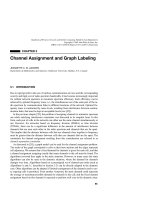
Figure 20.10 shows a sample multicast initiated from node 11, where MG = {4, 5, 6,
9}. Source 11 first sends multicast packets to the source gateway 8, where the initial FT is
generated [see Figure 20.10 (b)]. Members in the member list that are not in the MG are
masked. Note that node 6 appears in the member list of both nodes 4 and 7. It is assumed
that node 6 is assigned to node 7 and, hence, it is masked in the member list of node 4.
When node 4 receives the incoming FT [see Figure 20.10 (c)], it finds out that in the entry
in which the next hop is 4, its destination is also 4; that is, node 4 is a leave. Because m
2

is
set (i.e., at least one nongateway neighbor of node 4 is in the multicast set), node 4 needs
to broadcast the packets once more to its nongateway neighbors.
Broadcast can be considered as a special case of multicast, so the above two approach-
es can also be used to carry out a broadcast. However, since broadcast covers all nodes in
the network, the flooding approach is more efficient. In flooding, whenever a node re-
ceives packets, it will forward them to all its neighbors (except the one along the incoming
channel) if the packets are not duplicates. However, straightforward broadcasting by
flooding is normally very costly and will result in serious redundancy, contention, and col-
lision. These problems are summarized in [24] and are called the broadcast storm prob-
lem. Stojmenovic, Seddigh, and Zunic [33] proposed significantly reducing or eliminating
the communication overhead of a broadcast by using the dominating set concept. Specifi-
cally, retransmissions by gateway nodes is sufficient. In addition, Rules 1 and 2 are modi-
fied by using node degrees instead of node IDs as primary keys in gateway node deci-
sions.
446
DOMINATING-SET-BASED ROUTING IN AD HOC WIRELESS NETWORKS
20.5 CONCLUSIONS AND FUTURE DIRECTIONS
In this chapter, we have proposed a simple and efficient distributed algorithm for calculat-
ing the connected dominating set in an ad hoc wireless network. When the transmission
radius of a mobile host is not too large, the proposed algorithm generates a small connect-
ed dominating set. Our proposed algorithm calculates connected dominating sets in O(⌬
2
)
time with distance-2 neighborhood information, where ⌬ is the maximum node degree in
20.5 CONCLUSIONS AND FUTURE DIRECTIONS 447
destination member list next hop distance m1 m2
destination member list next hop distance m1 m2
sender = {11}
receiver = {4,5,6,9}

FG = {7,8}
FT and Mcast data flow
Mcast data flow
01
10
11
9()
4 (5)
9
7
1
2
(b)
(a)
2
1
11
10
7
8
5
9
4
6
3
(c)
(5) 4 1
(6) 7 1
11
01

(6) 7 17
7
4
Figure 20.10 (a) A sample multicast in an ad hoc wireless network. (b) The FT of node 8. (c) The
FT of node 7.
the graph. In addition, the proposed algorithm uses constant (1 or 2) rounds of message
exchange, compared with O(
␥
) rounds of message exchange in many existing approaches,
where
␥
is the domination number. The search space for a routing process can be reduced
to an induced graph generated from the connected dominating set.
One future direction of dominating-set-based routing is to integrate it with existing ap-
proaches. For example, the dominating set concept can be used together with location in-
formation obtained via geolocation techniques such as GPS. Some preliminary results
have been reported in [9] and [32].
ACKNOWLEDGMENTS
This work was supported in part by NSF grants CCR 9900646 and ANI 0073736. The au-
thor wishes to thank Hailan Li, who participated in the early stage of this project. The au-
thor can be reached at
REFERENCES
1. T. Ballardie, P. Francis, and J. Crowcroft, Core based trees (CBT): An architecture for scalable
inter-domain multicast routing, Proceedings of ACM SIGCOMM’93, p. 85, 1993.
2. J. A. Bondy and U. S. R. Murty, Graph Theory with Applications, Amsterdam: North-Holland,
1976.
3. J. Broch, D. B. Johnson, and D. A. Maltz, The Dynamic Source Routing Protocol for Mobile Ad
Hoc Networks, IETF, Internet Draft, draft-ietf-manet-dsr-00.txt,, 1998.
4. C C. Chiang, Routing in clustered multihop, mobile wireless networks with fading channels,
Proceedings of IEEE SICON’97, p. 197, 1997.

5. C C. Chiang, M. Gerla, and L. Zhang, Forwarding group multicast protocol (FGMP) for multi-
hop, mobile wireless networks, Cluster Computing, 1, 2, 187, 1998.
6. B. Das, E. Sivakumar, and V. Bhargavan, Routing in ad hoc networks using a virtual backbone,
Proceedings of the 6th International Conference on Computer Communications and Networks
(IC3N’97), 1997.
7. B. Das, E. Sivakumar, and V. Bhargavan, Routing in ad hoc networks using a spine, IEEE Inter-
national Conference on Computers and Communications Networks (ICC’97), 1997.
8. B. Das and V. Bhargavan, Routing in ad hoc networks using minimum connected dominating
sets, IEEE International Conference on Communications (ICC’97), 1997.
9. S. Datta, I. Stojmenovic, and J. Wu, Internal nodes and shortcut cased routing with guaranteed
delivery in wireless networks, in Proceedings of the International Workshop on Wireless Net-
works and Mobile Computing (in conjunction with ICDCS 2001), p. 461, 2001.
10. S. E. Deering and D. R. Cheriton, Multicast routing in datagram internetworks and extended
LANs, ACM Transactions on Computer Systems, 8, 85, 1990.
11. D. Estrin, R. Govindan, J. Heidemann, and S. Kumar, Next century challenges: Scalable coordi-
nation in sensor networks, Proceedings of ACM MOBICOM’99, p. 263, 1999.
12. IEEE Standards Departments, IEEE Draft Standard—Wireless LAN, New York: IEEE Press,
1996.
448
DOMINATING-SET-BASED ROUTING IN AD HOC WIRELESS NETWORKS
13. S. Guha and S. Khuller, Approximation algorithms for connected dominating sets, Algorithmi-
ca, 20, 4, 374, 1998.
14. T. W. Haynes, S. T. Hedetniemi, and P. J. Slater, Fundamentals of Domination in Graphs, New
York: Marcel Dekker,, 1998.
15. C. Hedrick, Routing Information protocol, Internet Request For Comments RFC 1058, 1998.
16. D. B. Johnson, Routing in ad hoc networks of mobile hosts, Proceedings of the IEEE Workshop
on Mobile Computing Systems and Applications, p. 158, 1994.
17. D. B. Johnson and D. A. Maltz, Dynamic source routing in ad hoc wireless networks, in Mobile
Computing, T. Imielinski and H. F. Korth (Eds.), Norwood, MA: Kluwer Academic Publishers,
p. 153, 1996.

18. J. Jubin and J. D. Tornow, The DARPA packet radio network protocols, Proceedings of the
IEEE, 75, 1, 21, 1987.
19. P. Krishna, M. Chatterjee, N. H. Vaidya, and D. K. Pradhan, A cluster-based approach for rout-
ing in ad hoc networks, Proceedings of the 2nd USENIX Symposium on Mobile and Location-
Independent Computing, p. 1, 1995.
20. C. R. Lin and M. Gerla, Adaptive clustering for mobile wireless networks, IEEE Journal on Se-
lected Areas in Communications, 15, 7, 1265, 1997.
21. J. M. McQuillan, I. Richer, and E. C. Rosen, The new routing algorithm for ARPANET, IEEE
Transactions on Communications, 28, 5, 171, 1980.
22. J. M. McQuillan and D. C. Walden, The ARPA network design decisions, Computer Networks,
1, 5, 243, 1977.
23. J. Moy, OSPF Version 2, Internet Request For Comments RFC 1247, 1991.
24. S. Y. Ni, Y. C. Tseng, Y. S. Chen, and J. P. Sheu, The broadcast storm problem in a mobile ad hoc
network, Proceedings of ACM MOBICOM’99, p. 151, 1999.
25. M. R. Pearlman and Z. J. Hass, Determining the optimal configuration for the zone routing pro-
tocol, IEEE Journal on Selected Areas in Communications, 17, 8, 1395, 1999.
26. C. E. Perkins and E. M. Royer, Highly Dynamic destination-sequenced distance-vector routing
(DSDV) for mobile computers, Proceedings of ACM SIGCOMM’94, p. 234, 1994.
27. R. Prakash, Unidirectional links prove costly in wireless ad hoc networks, Proceedings of the
3rd International Workshop on Discrete Algorithms and Methods for Mobile Computing and
Communications, p. 15, 1999.
28. C. Rohl, H. Woesner, and A. Wolisz, A short look on power saving mechanisms in the wireless
LAN Standard Draft IEEE 802.11, Proceedings of the 6th WINLAB Workshop on Third Genera-
tion Wireless Systems, 1997.
29. E. M. Royer and C. -K. Toh, A review of current routing protocols for ad hoc mobile wireless
networks, IEEE Personal Communications,6, 2, 46, 1999.
30. R. Sivakumar, B. Das, and V. Bhargavan, An improved spine-based infrastructure for routing in
ad hoc networks, Proceedings of the International Symposium on Computers and Communica-
tions (ISCC’98), 1998.
31. M. Steenstrup, Routing in Communications Networks, Upper Saddle River, NJ: Prentice Hall,,

1995.
32. I. Stojmenovic and X. Lin, GEDIR: Loop-free location based routing in wireless networks,
IASETED International Conference on Parallel and Distributed Computing and Systems, p.
1025, 1999.
REFERENCES 449