Tài liệu Sổ tay của các mạng không dây và điện toán di động P21 pdf

CHAPTER 21
Location Updates for Efficient Routing
in Ad Hoc Networks
IVAN STOJMENOVIC
´
DISCA, IIMAS, UNAM, Universidad Nacional Autonoma de Mexico
21.1 INTRODUCTION
Mobile ad hoc networks consist of wireless hosts that communicate with each other in the
absence of a fixed infrastructure. Some examples of the possible uses of ad hoc network-
ing include soldiers on the battlefield, emergency disaster relief personnel, and networks
of laptops. Sensor networks are a similar kind of network that have recently been investi-
gated. Nodes in a sensor network are lighter, computationally less powerful, and more
likely to be static compared to nodes in an ad hoc network. Hundreds or thousands of such
nodes may be placed to monitor and control a physical environment from possibly remote
locations. These nodes frequently switch their activity status to preserve battery power,
which poses additional challenges for the design of efficient data collection algorithms.
Ad hoc and sensor networks are self-organized and collaborative. Zero configuration net-
working is also required for environments in which administration is impractical or im-
possible, such as home or small offices or embedded systems “plugged together” (as in an
automobile), or for allowing impromptu networks between the devices of strangers on a
train [50].
In this chapter, we consider the routing task in which a message is to be sent from a
source node to a destination node. Due to propagation path loss, the transmission radii are
limited. Thus, routes between two hosts in a network may consist of hops through other
hosts in the network. The task of finding and maintaining routes in the network is nontriv-
ial since host mobility causes frequent unpredictable topological changes. “Sleep period
operation” (when some nodes become temporarily inactive) poses additional challenges
for routing protocols.
Macker and Corson [35] listed qualitative and quantitative independent metrics for
judging the performance of routing protocols. Desirable qualitative properties include:
distributed operation, loop-freedom (to avoid the worst-case scenario of a small fraction

of packets spinning around in the network), demand-based operation, and “sleep period
operation.” Some quantitative metrics that are appropriate for assessing the performance
of any routing protocol include [35] end-to-end data delay and average number of data bits
(or control bits) transmitted per data bits delivered. Our review (with primary interest in
451
Handbook of Wireless Networks and Mobile Computing, Edited by Ivan Stojmenovic´
Copyright © 2002 John Wiley & Sons, Inc.
ISBNs: 0-471-41902-8 (Paper); 0-471-22456-1 (Electronic)
location-based techniques) indicates that most proposed routing algorithms (more precise-
ly, their performance evaluations) ignore one or more of these important metrics.
Ad hoc networks are best modeled by minpower graphs constructed in the following
way. Each node A has its transmission range t(A). Two nodes A and B in the network are
neighbors (and thus joined by an edge) if the Euclidean distance between their coordinates
in the network is less than the minimum between their transmission radii (i.e., d(A, B) <
min {t(A), t(B)}. If all transmission ranges are equal, the corresponding graph is known as
the unit graph. In the unit graph model, forwarded messages simultaneously provide ac-
knowledgments for received messages. The minpower and unit graphs are valid models
when there are no obstacles in the signal path (e.g., a building). Ad hoc networks with ob-
stacles can be modeled by subgraphs of minpower or unit graphs. Most papers use unit
graphs for the performance evaluation of proposed routing protocols.
In the next section, we classify existing routing algorithms according to a number of
criteria. This section will also review a number of routing protocols. In Section 21.3, loca-
tion updates between neighboring nodes are discussed. Sections 21.4 through 21.7 de-
scribe several existing location update methods. Priority is given to newer algorithms with
novel approaches. Performance evaluation issues are discussed in Section 21.8. The refer-
ence section gives an extensive list of relevant articles.
21.2 CLASSIFICATION OF ROUTING ALGORITHMS
We shall now review the main characteristics of proposed routing algorithms in light of
desired qualitative and quantitative properties [35] and a few additional characteristics.
21.2.1 Demand-Based Operation

Routing algorithms can be classified as proactive or reactive. Proactive protocols maintain
routing tables when nodes move, independently of traffic demand, and thus may have un-
acceptable overhead when data traffic is considerably lower than mobility rate. For in-
stance, shortest- (weighted) path-based-solutions [3, 43, 45] are too sensitive to small
changes in local topology and activity status (the later even does not involve node move-
ment). The communication overhead involved in maintaining global information about the
networks is not acceptable for networks whose bandwidth and battery power are severely
limited. They are not elaborated on further in this chapter.
Routes in reactive algorithms are established when they are needed, in order to mini-
mize the communication overhead. They are adaptive to “sleep period” operation, since
inactive nodes simply do not participate at the time the route is established. One of well-
known reactive algorithms is the source-initiated, on-demand routing strategy [5, 22, 41,
44, 45]. In this strategy, the source or intermediate node S issues destination search re-
quest if the route to destination D is not available. The destination search is performed by
flooding a “short” search message, so that each node in the network is reached. Flooding
algorithms that reduce the number of retransmissions are surveyed and discussed in [50].
The path to destination is memorized in the process [5, 22, 41, 44, 45]. A variant of this
strategy is proposed in [53]. Several search “tickets” (each ticket is a “short” message con-
452
LOCATION UPDATES FOR EFFICIENT ROUTING IN AD HOC NETWORKS
taining the sender’s ID and location, the destination’s ID and best-known location and time
when that location was reported, and a constant amount of additional information) that
will look for the exact position of the destination node are issued by source S. When the
first ticket arrives at the destination node D, D will report back to the source with a brief
message containing its exact location, and possibly create a route for the source (the sec-
ond phase). In the third phase, the source node then sends a full data message (“long”
message) toward the exact location of destination. The efficiency of destination search de-
pends on the corresponding location update scheme. A quorum-based, home-agent-based,
and depth-first-search-based destination search and corresponding location update
schemes are being developed [49, 53, 54]. Other location update and destination search

schemes may be used, including an occasional flooding. If the routing problem is divided
as described, the mobility issue can be algorithmically separated from the routing issue,
allowing the application of routing algorithms with known destination in the second and
third phases of the protocol. The choice is justified whenever the destination does not
move significantly between its detection and message delivery, and information about
neighboring nodes is regularly maintained. In the described approach, the communication
overhead of routing algorithm is divided into the following components: location updates,
destination searches (performed in accordance to location update scheme), and path cre-
ation (or reporting from destination back to source).
An interesting compromise between proactive and reactive methods is proposed in [7].
The algorithm is destination-initiated: a destination initiates a global path computation to
itself using dynamic link metrics, which include a measure of “hotness” of the particular
destination and congestion in the vicinity of the destination. The updated routes are short-
est cost path routes, where queue length at each link (which is proportional to delay) is
taken as the cost measure.
21.2.2 Distributed Operation
We shall divide all distributed routing algorithms into localized and nonlocalized. Local-
ized algorithms [12] are distributed algorithms that resemble greedy algorithms in which
simple local behavior achieves a desired global objective. In a localized routing algorithm
[4, 6, 14, 28, 29, 47–49, 55], each node makes the decision of which neighbor to forward
the message based solely on the location of itself, its neighboring nodes, and the destina-
tion. Although neighboring nodes may update each other’s location whenever an edge is
broken or created, the accuracy of destination location is a serious problem. In some cases
such as monitoring the environment by sensor networks, the destination is a fixed node
known to all nodes (i.e., monitoring center). Localized algorithms are directly applicable
in such environments. Otherwise, they may use destination search as the first step, routing
short messages from destination to source as the second, and, finally, routing full message
from source to destination. Localized routing algorithms that guarantee delivery [6, 11]
(assuming that the destination location is accurate and message transmissions by nodes on
the route do not collide with other traffic) show that localized algorithms can nearly match

the performance of shortest path algorithms. All nonlocalized routing algorithms pro-
posed in the literature are variations of shortest weighted path algorithm [3, 5, 9, 22, 32,
41, 43]. Zone-based approaches combining shortest paths within a zone and interzonal
21.2 CLASSIFICATION OF ROUTING ALGORITHMS 453
destination searches or routing tables are elaborated in [23, 33]. In zone-based routing al-
gorithms [23], nodes are divided into nonoverlapping zones. Each node only knows node
connectivity within its own zone, and routing within the zone is performed directly. If the
destination is outside the zone, one location request is sent to every zone to find the desti-
nation. This seems to add significant overhead, indicating that combined requests in this
planar interzonal graph should be designed instead. Additional problems may arise when
nodes within the same zone are disconnected and neighboring zones are not reachable
from all nodes within a zone. Thus, this promising protocol needs further development. A
zone-based protocol that does not use location information of nodes is described in [21].
GRID protocol [33] selects one node in each grid or zone, and these nodes serve as the
backbone for routing tasks.
21.2.3 Location Information
Most proposed routing algorithms do not use the location of nodes, that is, their coordi-
nates in two- or three-dimensional space, in routing decisions [5, 23, 44, 45]. The distance
between neighboring nodes can be estimated on the basis of incoming signal strengths (if
some control messages are sent using fixed power). Relative coordinates of neighboring
nodes can be obtained by exchanging such information between neighbors. Alternatively,
the location of nodes may be available directly by communicating with a satellite through
GPS (Global Positioning System) if nodes are equipped with a small low-power GPS re-
ceiver. We believe that the advantages of using location information outweigh the cost of
additional hardware, if any. The distance information, for instance, allows nodes to adjust
their transmission powers and reduce transmission power accordingly. This enables using
power, cost, and power cost metrics [10, 43, 48] and corresponding routing algorithms
[48] in order to minimize energy required per routing task and to maximize the number of
routing tasks that a network can perform. Routing tables that are updated by mobile soft-
ware agents modeled on ants are used in [8]. Ants collect and disseminate location infor-

mation about nodes.
21.2.4 Single-Path versus Multipath Strategies
There exist several multipath, full-message strategies in which each node on the path
sends a full message to several neighbors that are best choices for all possible destina-
tion positions [4]. There is significant communication overhead, and lack of guaranteed
delivery can make this approach inferior to even a simple flooding algorithm. Clever
flooding algorithms may use about half of the nodes only for retransmissions [50],
which often matches the number of nodes participating in routing in this method. In ad-
dition, flooding guarantees delivery and requires no prior location updates for improved
efficiency. In [20], it was argued that flooding is the best routing method for very high
mobility rates. Multipath methods [4, 29, 52] may be regarded as flooding that is re-
stricted to the request zone and, as such, can be used for geocasting (in which a message
is to be delivered to all nodes located within a region). A multipath algorithm that con-
sists of several single paths is proposed in [47]. A single nonoptimal path, full-message
strategy is proposed in [1]. A short message, multipath destination search, full-message,
454
LOCATION UPDATES FOR EFFICIENT ROUTING IN AD HOC NETWORKS
optimal singlepath method was discussed above. The localized algorithms in this cate-
gory will be briefly described below.
Several GPS-based methods were proposed in 1984–1986 using the notion of progress.
Define progress as the distance between the transmitting node and receiving node project-
ed onto a line drawn from the transmitter toward the final destination. A neighbor is in the
forward direction if the progress is positive; otherwise it is said to be in the backward di-
rection. In the random progress method [38], packets destined toward D are routed with
equal probability toward one neighboring node that has positive progress. In the NFP
method [17], a packet is sent to the nearest neighboring node with forward progress. Taka-
gi and Kleinrock [35] proposed the MFR (most forward within radius) routing algorithm,
in which a packet is sent to the neighbor with the greatest progress. The method is modi-
fied in [17] by proposing to adjust the transmission power to the distance between the two
nodes. Finn [14] proposed a Cartesian routing method that allows choosing any successor

node that makes progress toward the packet’s destination. The best choice depends on the
complete topological knowledge. Finn [14] adopted the greedy principle in his simulation:
choose the successor node that is closest to the destination. When no node is closer to the
destination than the current node, the algorithm performs a sophisticated procedure that
does not guaranty delivery. Recently, three articles [4, 28, 29] independently reported vari-
ations of routing protocols based on direction of destination. In the compass routing (or
DIR) method proposed by Kranakis, Singh, and Urrutia [28], the source or intermediate
node A uses the location information for the destination D to calculate its direction. The
location of one-hop neighbors of A is used to determine for which of them, say C, the di-
rection AC is closest to the direction of AD. The message m is forwarded to C. The process
repeats until the destination is, hopefully, reached. The GEDIR routing algorithm [47] is a
variant of greedy routing algorithm [14] with a “delayed” failure criterion. GEDIR, MFR,
and compass routing algorithms fail to deliver messages if the best choice for a node cur-
rently holding a message is to return it to the previous node [47]. A GFG routing algo-
rithm that guarantees delivery by finding a simple path between source and destination is
described in [6]. It is based on constructing a planar subgraph (e.g., Gabriel graph) and
providing routing in the planar subgraph that guarantees delivery. This procedure is called
on whenever the greedy algorithm fails, and is recalled whenever a closer node (than the
previously failing node) is encountered. The GFG algorithm [6] was implemented in [26]
by including MAC layer considerations and location updates for experiments with moving
nodes. The performance of the GFG algorithm was improved in [11] by adding a shortcut
procedure and applying the internal node concept of Wu and Lee [57]. The hop count is
very close to the hop count of the shortest path algorithm for dense graphs (below 20%
excess hop count for graphs with average degrees Ն6) and about twice as long for sparse
graphs. Corresponding power- and cost-aware routing algorithms with guaranteed deliv-
ery are developed in [46].
21.2.5 Loop Freedom
Interestingly, loop freedom, a basic criterion of Macker and Corson [35] was neglected in
many papers. GEDIR and MFR algorithms are inherently loop-free [47]. The proofs of
this are based on the observation that distances (or dot products) of nodes toward the des-

21.2 CLASSIFICATION OF ROUTING ALGORITHMS 455
tination are decreasing. A counterexample showing that undetected loops can be created in
directional-based methods [4, 28, 29] is given in [47]. The method is therefore not loop-
free. The algorithms in [6, 11, 14, 35] and shortest-weighted-path-based routing schemes
are loop-free.
21.2.6 Memorization of Past Traffic
Most reported algorithms require some or all nodes to memorize past traffic as part of
current the routing protocol or to memorize the previous best paths for providing future
path to the same destination. Solutions that require nodes to memorize routes or partic-
ular information about past traffic are sensitive to node queue size and changes in node
activity and node mobility while routing is ongoing. One form of such memorization is
provided by routing tables, which memorize the last successful path to each destination.
Reduction in the size of routing tables (and, consequently, in the communication over-
head to maintain them) was proposed in [25, 57] by defining backbone structures. Each
node in the network is either in the virtual backbone or at most r hops away from a vir-
tual backbone node. Clustering has frequently been used to provide such a backbone
[25], where the r-cluster is defined as the set of all the nodes within distance at most r
hops from a given node, referred to as the clusterhead of the r-cluster. Border nodes are
nodes that belong to two or more clusters. Clusterheads are backbone nodes, and two
“neighboring” backbone nodes may be up to 2r + 1 hops away. Thus, communication be-
tween two backbone nodes may go through both backbone and nonbackbone nodes. A
distributed scheme for initiating is based on selecting, repeatedly, a node with a maximal
number of unassigned r hop neighbors as the backbone node, and assigning all its r hop
neighbors to that node. Such a backbone is also used in the routing algorithm [30]. The
maintenance of cluster structure is known to require significant communication overhead
(for instance, local changes may cause global updates by the chain effect) [57]. A sig-
nificantly better backbone structure, one that does not require any communication over-
head and provides connectivity between nodes, is described in [57] and is based on sev-
eral definitions of dominating sets.
Localized routing algorithms discussed above [6, 14, 28, 46–48, 55] do not memorize

past traffic at any node. The algorithms [4, 29, 52] require nodes to memorize past traffic
to avoid infinite mutual flooding between neighboring nodes. Memorization of escape
loops is needed in directional-based methods (alternatively, messages need to carry time-
out stamps). In flooding GEDIR and MFR algorithms [47], messages are flooded at nodes
in which basic algorithms fail, and these nodes refuse further copies of the same message.
These algorithms guaranty delivery. Routing algorithms that use depth-first search (DFS)
in the search for destination are discussed in [24, 49]. Memorization here is imposed by
the DFS process. The algorithm guarantees delivery but the efficiency depends on the ac-
curacy of the destination information. Memorization is needed in sensor networks for data
fusion [12] to avoid multiple reports of the same information. Quality of service routing,
in which the path needs to satisfy delay, bandwidth, and connection time criteria [49], re-
quires that nodes memorize the QoS path; thus, using DFS for its construction does not
impose any memorization overhead.
456
LOCATION UPDATES FOR EFFICIENT ROUTING IN AD HOC NETWORKS
21.3 LOCATION UPDATES BETWEEN NEIGHBORING NODES
One of most important ingredients in all location update schemes is the update between
neighboring nodes. The question is when does a node decide to send a message to all its
neighbors announcing its new location. We shall review the methods used in literature. As
a basic (or “bonus”) update, nodes may update their location information with each ex-
change of routing messages between them.
Karumanchi, Muralidharan, and Prakash [27] discussed the question when to update
location, and argued that distance-based updates (based on absolute distance traveled
since the last update) and movement-based updates (based on the velocities of nodes) may
have limited usefulness in ad hoc networks (such location updates are used in [4, 29]). For
instance, nodes may move within a small circle, causing unnecessary location updates.
They concluded experimentally that the best strategy is to update when a certain prespeci-
fied number of links incident on a node have been established or broken since the last up-
date [27].
The basic update procedure is performed by each moving node whenever it observes

that, due to its movement, an existing edge will be broken (that is, the distance between
two nodes becomes >R). In order to minimize the number of location update messages,
the message could be sent by only the node endpoint (of the broken edge) with greater
speed. Similarly, the same action may be taken when a new neighbor is detected. New
neighbor X may be detected after X transmitted its location update following an edge
breakup with another node. Thus, new neighbors that receive such messages may then re-
act by informing X about their presence. Alternatively, the creation of a new link can be
detected if two-hop information is available to nodes.
To decide whether an edge is made or broken, a node may use last available informa-
tion about its direct neighbors and other nodes in the network. However, when all nodes
are moving in the same direction (as in military or rescue missions), such a procedure may
result in unnecessary updates. To reduce overhead in such scenarios, connection time is
introduced as follows. The availability of GPS enables nodes to estimate the connection
time with other nodes, as proposed in [49, 51]. The connection time is defined as the esti-
mated duration of a connection between two neighboring nodes. Neighboring nodes fre-
quently update their location to each other, and this information may be used to estimate
the direction and speed of their movements. In turn, this suffices to estimate the connec-
tion time. Let A and B be the two neighboring nodes that move at speeds a and b, respec-
tively. Here, A and B are position vectors and a and b are directional vectors. At time t,
they move to new positions AЈ = A + at and BЈ = B + bt. They will loose their connection
when the distance between them becomes >R, where R is the radius of the corresponding
unit graph (or the smaller of their transmission radii in case of minpower graphs). The
time t at which the connection will be lost can be estimated by solving the quadratic equa-
tion |AЈBЈ| = |B – A + (b – a)t| = R [49, 51]. When the time expires, the edge is assumed to
broken and a location update is sent to all neighbors. Similar criteria can be used to esti-
mate the time a connection will be made, and act accordingly.
The variants of this basic update may include adjusting transmission radius to tR for
some value of t, to reach more or fewer neighbors. Location updates are short messages,
21.3 LOCATION UPDATES BETWEEN NEIGHBORING NODES 457
and nodes may spend more energy for short messages, as suggested by Lin and Liu [32].

They discussed this difference and even proposed an extreme difference in radii for short
and long messages. They found that nodes are able to send their new location to all other
nodes in a network with a single broadcast (single-hop network for location updates).
However, when sending exact data, the network is treated as a multihop one. Note that the
single-hop location update broadcast may fail to reach a number of nodes due to obstacles
in the field or presence of other transmissions. Another possible solution is to keep the
transmission radius at R, but retransmit from each of the neighbors that are a few hops
away. However, these retransmissions also require power (from neighboring nodes), and
may cause the broadcast storm problem [NTCS]; therefore, their efficiency is doubtful.
Note that a node that receives a location update aimed at known neighboring nodes, and
discovers that it is now a neighbor of transmitting node that is not aware of it, will treat this
event as the creation of a new edge and react by sending its own location update in response.
This basic location update procedure may be used as a counter for “deeper” location
updates. For instance, Basagni et al. [4] used parameter p (the distance traveled from the
last update) as such a counter. Two-hop, four-hop, and flooding messages are sent on
every first, second, and third counter, respectively.
21.4 REQUEST ZONE ROUTING
A distance routing effect algorithm for mobility (DREAM) is described in [4]. The source
or any intermediate node A calculates the direction of destination D and, based on the mo-
bility information about D, chooses an angular range. The message m is forwarded to all
neighbors whose direction belongs to the selected range. The range is determined by the
tangents from A to the circle centered at D, with radius equal to a maximal possible move-
ment of D since the last location update. The area containing the circle and two tangents is
referred as the request zone [29]. Ko and Vaidya [29] described, independently, an almost
identical algorithm, called the LAR Scheme 1, and a few modifications of it. The modifi-
cations include sending route requests before the message itself [22]. Note that a route re-
quest may be considered as a routing of short messages, as discussed above. Recovery
procedures, based on partial or full flooding, to start flooding if the given algorithm fails
to find the route within a timeout interval, are proposed in both papers [4, 29]. Ko and
Vaidya [29] also proposed the LAR Scheme 2. In this scheme, the source or each interme-

diate node A will forward the message to all nodes that are closer to the destination than A
is. Wu and Harms [56] proposed to improve the location update part of the LAR algo-
rithm. In [56], any two neighboring nodes periodically exchange full routing table (infor-
mation about all nodes in the network).
The definition of the request zone [4, 29] was modified in [52] in order to provide a
uniform framework with the corresponding notions in GEDIR and MFR methods. Stoj-
menovic [52] discusses the V-GEDIR, CH-MFR, and R-DIR methods, in which m is for-
warded to exactly those neighbors that may be the best choices for a possible position of
destination (using the appropriate criterion). The request zone in the R-DIR method [52]
may include one or two neighbors that are outside of angular range, because they can have
the closest direction for the tangents to the circle. In the V-GEDIR method, these neigh-
458
LOCATION UPDATES FOR EFFICIENT ROUTING IN AD HOC NETWORKS
bors are determined by intersecting the Voronoi diagram of neighbors with the circle (or
rectangle) of possible positions of destination; the portion of the convex hull of neighbor-
ing nodes is analogously used in the CH-MFR method.
The Voronoi diagram of n distinct points in the plane is a partition of the plane into n
Voronoi regions, each one associated with each point. The Voronoi region associated with
node A consists of all the points in the plane that are closer to A than to any other node. It
can be shown that each region is a convex polygon (possibly unbounded) determined by
bisectors of A and other nodes (more precisely, each region is the intersection of all such
bisectors). It is well known that the Voronoi diagram for n points in the plane can be con-
structed in O(n log n) time [40] and consists of O(n) line segments.
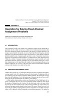
Node S, currently holding a message for destination D, computes the Voronoi diagram
of all its n neighbors. For example, in Figure 21.1, the Voronoi diagram of five neighbors
A, B, C, E, and F is shown in dashed lines. Consider the circle (or other region) where des-
tination D can be located. Different locations of D inside the circle correspond to different
choices of closest nodes among A, B, C, E, and F. For each position of D, the closest node
is the one whose Voronoi region contains the position. Thus, the nodes that are closest to
some positions of destination are exactly those nodes whose Voronoi regions intersect the

circle of possible destination positions (e.g., B and E in Figure 21.1).
21.5 DOUBLING CIRCLES ROUTING
Amouris, Papavassiliou, and Lu [1] presented a position-based, multizone routing proto-
col for wide area mobile ad hoc networks. Their algorithm is based on position updates
within circles of increasing radii. Each node updates its location to all nodes located with-
in a circle of radii P, 2P, 4P, 8P, . . . (each subsequent circle has a twice larger radius than
21.5 DOUBLING CIRCLES ROUTING 459
Figure 21.1 Voronoi diagram and the request zone.
the previous one). Whenever a given node A moves outside one of these circles of radius
2
t
P for some t, node A broadcasts its location update to all nodes located inside a circle
centered at the current node position and with radius 2
t+1
P. The routing toward destination
then follows these circles of last updates. Source nodes send messages toward the last re-
ported position of destination (using the DIR method) that has moved within the circle of
some radius since the last report. As routing the message moves closer to the destination,
the information about position of destination becomes more precise, and nodes are able to
send messages toward the centers of circles with twice smaller radii than previously, until
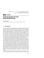
the node is eventually reached. This process is illustrated in Figure 21.2. The source S
sends a message toward DЈ, the last known position of destination D. The routing is later
redirected toward newer position DЈ and finally to exact position D. This method is very
interesting and certainly competitive. We observe that the radii of larger circles may en-
compass almost all nodes of the network, and that the routing paths discovered by the al-
gorithm do not have near-optimal hop counts (which may be important in quality of ser-
vice applications). However, if the path quality is important, one can consider this
algorithm only as the destination search step in the three-phase routing algorithm de-
scribed above. A similar algorithm, using squares instead of circles and additional sophis-
ticated techniques, is proposed in [31].

The location update techniques discussed so far include occasional flooding of location
information to all or a large portion of nodes in the network. In the next two sections,
methods that never use such flooding are discussed.
21.6 QUORUM-BASED STRATEGIES
Quorum-based approaches for information dissemination are based on replicating infor-
mation at multiple nodes acting as repositories. The choice of repositories and the query
460
LOCATION UPDATES FOR EFFICIENT ROUTING IN AD HOC NETWORKS
Figure 21.2 Routing from S toward DЈ, DЈЈ, and D.
search must be mutually compatible. Such query and update strategies have been previ-
ously employed for location management in cellular networks. Given a set S of n servers, a
quorum system is a set of mutually disjoint subsets of S whose union is S. When one of
servers requires information from the other, it suffices to query one server from each quo-
rum. In fixed networks, the set of queried servers is bound to contain at least one server
that belonged to the quorum that received the latest update. Hence, each query returns the
latest value of the queried data. It is possible to form quorums of size approximately n
1/2
[34]. For example, 25 servers can be organized into 5 rows and 5 columns. Each column
serves as a quorum. Thus each node (i, j) (located in i-th row and j-th column) replicates
its data to all servers (iЈ, j) in its column. To extract the information from server (i, j), serv-
er (iЈ, jЈ) may inquire within its iЈ-th row, and the server (iЈ, j) will provide the requested
information. Modifications of quorum-based strategies for use in dynamic or partitionable
servers have been considered in [13, 16, 18, 19, 27, 30]. The main idea in [13, 16, 27] is
that each server (or node) selects one of the quorums at random to increase the chance of
obtaining relatively up-to-date information in several “columns.”
Karumanchi, Muralidharan, and Prakash [27] discussed information dissemination in
partitionable mobile ad hoc networks. They studied the problem of getting the location of
some other node in the network and the surroundings of that node (e.g., firefighter) with-
out the need to route any message to that node. Their performance evaluation is limited in
measuring the accuracy of the obtained information (i.e., the distance between the found

and exact location of the other node). In [27], n nodes are divided into n
1/2
groups with n
1/2
nodes in each, in two ways, and such quorums are preserved while moving.
Haas and Liang [18, 19, 30] proposed another variant of the quorum-based distributed
mobility management scheme. First, a virtual backbone [25, 30] is initiated and main-
tained. Nodes in the virtual backbone are database servers for location information. They
define a quorum system, that is, a set of subsets such that any two subsets intersect in a
small number (preferably constant number t) of databases. Each subset then has the same
size k. In [18] the choice of subsets is uniform and is performed by applying a centralized,
balanced, incomplete block design algorithm. The random selection of these subsets was
discussed in [19]. When a node moves, it updates its location, with one subset containing
the nearest backbone node. Each source node then queries the subset containing its nearest
backbone for the location of the destination, and uses that location to route the message.
The routing algorithm is not discussed in [18, 19, 30]. It can be easily observed that loca-
tion updates and destination searches are not local, and that they involve routing between
backbone nodes. Thus, backbone nodes must exchange their location information in order
to perform their duties. It is not clear, taking all the overhead into account, whether the
whole algorithm will perform better than a simple flooding algorithm with redundant re-
transmissions eliminated [50]. The flooding algorithm does not require any location up-
dates, and does not require communication overhead for its own backbone structure,
which is the dominating set, as defined in [57]. In particular, the same backbone structure
can be used for efficient flooding [50] and efficient routing [57].
The main problem with the described quorum-based strategies is that quorums are
themselves fixed, and movement of nodes can make nodes in the same quorum far apart
from each other, with no clear way of visiting them all in order to find destination infor-
mation that may be no more difficult to find than the other nodes in the same quorum. A
different quorum-based strategy, which deals with network dynamics, is proposed in [53].
21.6 QUORUM-BASED STRATEGIES 461

In [53], nodes in an ad hoc network do not stay in the same “column,” and the distributed
information may easily disperse due to node movement. Moreover, it is not clear what the
“column” is, and how all the nodes in a column, once defined, will receive the latest up-
dates. Nevertheless, we believe that this idea is worth pursuing.
The main location update method is to forward the new location information (and the
node’s identifier) within a “column” in the network, in the following way. Each node uses
a counter to count the number of previously made changes in edge existence (the number
of created or broken edges). When the counter reaches a fixed threshold value e, location
information is forwarded along the “column” and e is reset to 0. The “column” may have
arbitrary “thickness,” but we shall assume, for clarity, thickness 1 here, which means that
the created column is a single path in the north–south direction, including neighbors of
nodes in that path. A initiates two routing messages, in the directions north and south,
whereas other nodes follow only one of the directions. Each follows variation of the MFR
algorithm [55], with destination always to the north (or south) of the current node, as fol-
lows. Current node B transmits update information to all its neighbors, and indicates, in
the same message, which of them is its northernmost (or southernmost) neighbor. That
node will, in turn, do the same until a node is reached that does not have such a neighbor.
The frequent problem with the scheme is that the northernmost node, as determined by
the northward update, may only be locally northernmost. A “horizontal” destination
search can miss such a node, which can remain “below” it. To overcome this problem,
each locally northernmost node may switch to FACE mode [6] until another, more north-
ern, node is found on a face. It then converts back to regular upward movement. This
switching can be repeated a few times. The FACE algorithm can be improved by applying
a shortcut scheme [11]. The final result will be that all nodes at the outer face of the net-
work will receive a location update. This method guarantees that “horizontal” destination
search and “vertical” location update will intersect at one of the nodes on the outer face.
The drawback is that nodes on the outer boundary will have more traffic demands.
The search for destination is performed similarly, using a horizontal east–west direc-
tion instead. The search message includes time of last available information, and other
nodes are requested to provide more up-to-date information, if they have it. Nodes that are

not on the horizontal path but receive the search message and have more up-to-date infor-
mation about destination will respond in the process with their information. Thus, data
link layer protocols should be efficient in such cases by avoiding collisions. When eastern-
most and westernmost nodes are reached (or the outer boundary is traversed if the FACE
algorithm is also incorporated), the search strategy changes. The message search is then
oriented toward the destination, using the latest available information for each search mes-
sage. There are three searches initiated. The first one originates at sender node S, using the
best locally available information. This search does not need to wait for the result of
searches in the east and west directions. The easternmost and westernmost nodes in a giv-
en “row” may initiate two other searches. Each of three search tasks follows a path toward
the destination, using the greedy/GEDIR strategy [14, 47] or GFG algorithm [6]. That is,
at each step, the neighbor closest to the destination is selected to forward the message.
Nodes that hear messages between two neighbors may react should they have better infor-
mation about the destination’s location.
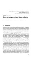
Figure 21.3 illustrates location update and destination search schemes. Destination
462
LOCATION UPDATES FOR EFFICIENT ROUTING IN AD HOC NETWORKS
node D moves (other nodes in Figure 21.3 are assumed to be static) from positions D1 to
D2 and finally to D3, and causes creation or breaking of some edges (indicated by arrows,
with nodes A1, A2, A3, and A4). At position D3, it decides to send a location update in its
current “column” by sending its position in the northern direction (it does so in the south-
ern direction as well, but there is no neighbor in that direction in Figure 21.3). The main
update path is indicated in bold lines, and bold, long dashed lines indicate some other
nodes that hear the update message. Source node S initiates a destination search in the
east–west direction (in Figure 21.3 it only has neighbors in western direction). The search
path is indicated by bold lines, whereas some other nodes, which observe the search, are
connected by short bold dashed lines. The location update column and destination search
row intersect in Figure 21.3 in seven nodes. The easternmost and westernmost points in
the row and node S then turn the search toward learned position of D. In Figure 21.3, point
W learned the up-to-date information and may find the destination by applying any local-

ized routing algorithm for static nodes (in Figure 21.3, GEDIR algorithm would produce
path W–B–C–A3–D3).
21.7 HOME-AGENT-BASED STRATEGY
The location update idea proposed in [2, 54] for mobile ad hoc or sensor networks is sim-
ilar to the one used in cellular phone networks and mobile IP. When a phone user moves
away from his home server (agent) to a new location, the visitor’s location periodically
sends messages to the home agent, giving its current coordinates. When a phone call is
made to that user, the call is first sent toward the user’s home agent. The home agent then
directs the call toward the visitor’s position.
The main location update procedure is performed by each node as follows [54]. At the
beginning, each node informs every other node about its initial position, which will be its
home agent. More precisely, the home agent will consist of all nodes that are currently lo-
21.7 HOME-AGENT-BASED STRATEGY 463
Figure 21.3 Location update from D3 and destination search from S.
cated inside a circle with radius pR, where p is network parameter, centered at the initial
position of the node. In [2], the fixed center of the home region is known by means of
some predefined hash function made aware of universally. The size of the home region in
[2] adapts to the density of the area, in order to maintain an approximately constant num-
ber of nodes inside the region. Each node A uses a counter to count the number of previ-
ously made changes in edge existence (the number of created or broken edges). When the
counter reaches a fixed threshold value e, node A sends a location update message to its
home agent using greedy/GEDIR [14, 47] or GFG [2] algorithm. Nodes on the path and
their neighbors also update information about A. If current node B is inside the home
agent base, the algorithm changes to flooding inside the home. Note that the update may
fail if home agent is disconnected from the current node location. Such failure may be re-
ported back to the node, which will then choose a new home.
Now suppose that source S wants to route a message to a destination D. Destination
search messages will be issued, looking for D. S sends exactly two such messages. One is
sent toward D using the location information about D currently available to S, applying
greedy or GFG algorithms. More up-to-date location information will be taken on the way

to the destination (if any is available). The second message is sent toward the center C of
the home agent circle of D, which may be at a different region than the current position of
D. The search message will stop in the same way as the location update message, at node
B, hopefully inside D’s home. Node B will then act on the basis of the best information
available, and redirect the message toward the location of the destination.
The location update and destination search schemes are illustrated in Figure 21.4. It
shows an ad hoc network with radius R, as indicated. Destination D is the only node that
moves (for clarity). D1, D2, and D3 are its positions during the move. Upon every link
464
LOCATION UPDATES FOR EFFICIENT ROUTING IN AD HOC NETWORKS
Figure 21.4 Location update from D2 and destination search from S.
change (making or breaking), D informs its neighbors (indicated by an arrow). At position
D2, it decides to inform its home agent, drawn as a circle, about its current position. The
location update message follows the path D2–U–V–W (indicated by a bold line), and is
broadcast from W to other nodes inside home agent circle (e.g., to nodes B and C, indicat-
ed by dotted lines). Now suppose that source S initiates a destination search when the des-
tination is at position D3. The destination search message is forwarded toward the center
of home agent circle and follows path S–K–I–H–G–L–M–N–B. Node B then forwards the
search message toward position D2, for which node P is the best neighbor (following a
GEDIR-like method). On the path B–P–Q–D3 (indicated by bold and long dashed lines),
node Q has the up-to-date location of D and the destination is found. The destination D
then initiates the path creation phase following the GFG algorithm [6] and finds the
source S using the path D3–A–E–F–G–H–I–K–S (indicated by bold lines). Source S may
then send the data toward D.
21.8 PERFORMANCE EVALUATION ISSUES
We shall now discuss the issues arising from performance evaluation of routing algo-
rithms. These will include quantitative metrics used, selection of parameters, comparison
with existing methods, mobility patterns, and selection of simulators.
21.8.1 Delivery Rate
The delivery rate is defined as the ratio of numbers of messages received by the destina-

tion and sent by senders. The best routing methods employing this metric are those that
guarantee delivery, such as [6], in which message delivery is guaranteed assuming “rea-
sonably” accurate destination and neighbor location and no message collisions.
21.8.2 End-to-End Data Delay
This is also referred to as latency, and is the time needed to deliver the message. Data delay
can be divided into queuing delay and propagation delay. If queuing delay is ignored, prop-
agation delay can be replaced by hop count, because of proportionality. Retransmissions
can be included if the MAC (medium access control) layer is used in experiments. Several
papers suggested that it is more important to minimize the power needed per message or the
number of routing tasks a network can perform before partitioning [10, 43, 48].
21.8.3 Communication Overhead
Communication overhead can be defined as the average number of control and data bits
transmitted per data bits delivered [35]. Control bits include the cost of location updates in
the preparation step and destination searches and retransmission during the routing
process. However, this metric is rarely used in the literature. In fact, most of the papers
avoid measuring it altogether. The portion of ignored overhead may often be more signifi-
cant than the measured one.
21.8 PERFORMANCE EVALUATION ISSUES 465
21.8.4 Performance on Static Networks
Although the algorithm is designed with moving nodes in mind, static nodes are important
special cases to be verified. Some networks, such as sensor networks, are static most of
time, and sometimes destination and neighbor information is accurate. How can one claim
that a routing algorithm that performs “well” on moving nodes (with carefully selected
moving patterns and network parameters) is a “winning” algorithm if it performs badly on
static networks? Experiments with static networks allow significant reduction of the num-
ber of parameters and simplification of experiments, thus “fine tuning” the algorithm be-
fore real experiments.
21.8.5 MAC Layer Considerations
Initial experiments may ignore the data link layer, but for similar reasons (in the absence
of message collisions, routing algorithms should have superb performance, e.g., guaran-

teeing delivery), further experiments, even on static networks, should consider it. A study
on whether the choice of MAC protocol affects the relative performance of the routing
protocols was done in [42]. Table-driven protocols are not affected significantly by the
choice of MAC protocol. Protocols with hello messaging, when run over IEEE 802.11,
have considerably less control traffic than when they run over CSMA (carrier sense multi-
ple access) or MACA (multiple access with collision avoidance). Therefore, IEEE 802.11
can be considered as a standard for MAC specifications in wireless networks.
21.8.6 Comparison with the Shortest Path Algorithm
There is a notable tendency in the literature to compare the performance of proposed rout-
ing algorithms with the worst possible solution—flooding—but such comparisons are not
properly done, since improper flooding algorithms are used. Algorithms that are able to
flood with reduced numbers of retransmissions (roughly half) are surveyed in [50]. If
flooding is used for comparison, then the proper version of it should be used. Although
some existing algorithms can also be used for comparison, especially if they belong to the
same class with the same classification criteria, the ideal shortest path (SP) algorithm is
certainly the ultimate goal, and one should verify how far from that goal the proposed al-
gorithm is. If the cost of location updates for both proposed and SP algorithms is ignored,
the flooding rate [47] (the ratio of the number of message transmissions and the shortest
possible hop count between two nodes) can be used for fair comparison, especially for
multipath methods. Each transmission in multiple routes is counted, and messages can be
sent to all neighbors with one transmission.
21.8.7 Generating Sparse and Dense Graphs
For experiments with static networks, random unit graphs should be generated. Each of n
nodes should select at random x and y coordinates in the interval [0 . . . m]. Subgraphs can
be used if obstacles are taken into account. The connectivity depends on the selected trans-
mission radius R. Since transmission radius R for a given piece of equipment is normally
466
LOCATION UPDATES FOR EFFICIENT ROUTING IN AD HOC NETWORKS
fixed (or should be selected from a few discrete values), most papers use a fixed value of R
and change m to evaluate graphs of different density (or, in many cases, fix m as well, with-

out discussing impact of graph density). Ignoring the graph density issue in performance
evaluations is the single most misleading point in the experimental design and interpreta-
tion of results. Routing algorithms perform differently on sparse and dense graphs; thus, it
is the graph density that is a primary independent variable to be considered. The best mea-
sure of graph density is the average number d of neighbors for each node. There is a relation
between R, m, and d, and one should choose d as independent variable. If R is fixed, then
change m accordingly. If m is fixed, then R can be found as follows [47]. Sort (in increasing
order) all n(n – 1)/2 possible edges in the graph and choose R to be equal to the length of the
nd/2-th edge in the sorted list. If R is to have a fixed value for some reason, adjust m linear-
ly with R, to keep the same underlying graph. Generated graphs that are disconnected may
or may not be eliminated (it is difficult to control full connectivity with moving nodes; ini-
tial connectivity does not secure connectivity during node movements).
21.8.8 Node Mobility
Some papers use random movements at each simulation step in four or eight possible di-
rections. Random walks tend to keep all nodes close to their initial positions, and thus
analysis using this model is largely misleading. We also believe that this is not a natural
kind of movement, and suggest using movement patterns as in [9, 22, 36]. One possible
analogous design is as follows. Each node generates a random number, wait, in interval [0
maxwait]. The node does not move for wait seconds. This is called the station time.
When this time expires, the node chooses to move with a probability p. It generates a new
wait period if it decides not to move. Otherwise, it generates a random number, travel, in
interval [0, maxtravel], and a new random position within the same square in the second
case. The node then moves from its old position to a new position along the line segment
joining them, at equal speed for the duration of travel seconds. Upon arriving at the new
location, the node again chooses its waiting period, etc. The mobility rate is given by the
formula mobrate = p*maxtravel/(maxtravel + maxwait) and is one of the main mobility
parameters. Note that this movement pattern does not cover the case of nodes moving
more or less in the same direction, which may often be the case in military and rescue op-
erations. Thus, an additional component should be added in experiments—moving with
the same speed and in the same direction by all nodes.

21.8.9 Simulators
There exist several wireless network simulators that are used in the literature. The two
most widely used are Glomosym [15] and ns-2 [37]. Although it is desirable to have some
kind of benchmark testing facility, the problem with these simulators is a painful learning
curve. Several researchers who have used it confirmed that it takes about one month of
full-time work to learn how to use these simulators. Thus, they may be a good choice for
long-term projects (and long-term grant holders), but not for researchers with limited hu-
man resources. The other drawback of using these simulators is that experiments with sta-
tic nodes and important parameters (e.g., graph density) are easily ignored. Preliminary
21.8 PERFORMANCE EVALUATION ISSUES 467
experiments with static nodes and even moving nodes can be obtained by a simplified de-
sign using any programming language (e.g., C or Java), and valuable conclusions can be
made. This should be done even if a simulator is used afterward. We agree, of course, that
real simulations are necessary for a complete performance evaluation, if resources for do-
ing so are available.
21.9 CONCLUSION
Our discussion indicates that the problem of routing in mobile wireless networks is far
from being solved, whereas the special cases of static networks, fixed destination, or
known location of destination seems to have been solved satisfactorily. We therefore ex-
pect that the research on location updates for efficient routing in wireless network will
continue, and hope that this chapter will provide a valuable source of information and di-
rections for future work and experimental designs.
REFERENCES
1. K. N. Amouris, S. Papavassiliou, and M. Li, A position based multi-zone routing protocol for
wide area mobile ad-hoc networks, Proceedings 49th IEEE Vehicular Technology Conference,
1999, pp. 1365–1369.
2. L. Blazevic, L. Buttyan, S. Capkun, S. Giordano, J P. Hubaux, and J Y. Le Boudec, Self-orga-
nization in mobile ad hoc networks: the approach of terminodes, IEEE Communication Maga-
zine, June 2001.
3. S. Basagni, I. Chlamtac, and V. R. Syrotiuk, Dynamic source routing for ad hoc networks using

the global positioning system, Proceedings IEEE Wireless Communications and Networking
Conference, New Orleans, Sept., 1999.
4. S. Basagni, I. Chlamtac, V. R. Syrotiuk, B. A. Woodward, A distance routing effect algorithm for
mobility (DREAM), Proceedings MOBICOM, 1998, pp. 76–84.
5. J. Broch, D. A. Maltz, D. B. Johnson, Y. C. Hu, and J. Jetcheva, A performance comparison of
multihop wireless ad hoc network routing protocols, Proceedings MOBICOM, 1998, pp. 85–97.
6. P. Bose, P. Morin, I. Stojmenovic, and J. Urrutia, Routing with guaranteed delivery in ad hoc
wireless networks, 3rd International Workshop on Discrete Algorithms and Methods for Mobile
Computing and Communications, Seattle, August 20, 1999, pp. 48–55.
7. J. Chen, P. Druschel, and D. Subramanian, A new approach to routing with dynamic metrics,
Proceedings IEEE INFOCOM, 1999.
8. D. Camara and A. F. Loureiro, A novel routing algorithm for ad hoc networks, Telecommunica-
tion Systems, to appear.
9. S. Chen and K. Nahrstedt, Distributed quality-of-service routing in ad hoc networks, IEEE
Journal Selected Areas in Communications, 17, 8, 1999, 1488–1505.
10. J. H. Chang and L. Tassiulas, Energy conserving routing in wireless ad-hoc networks, Proceed-
ings IEEE INFOCOM, March, 2000.
11. S. Datta, I. Stojmenovic, and J. Wu, Internal node and shortcut based routing with guaranteed
delivery in wireless networks, Cluster Computing, to appear.
468
LOCATION UPDATES FOR EFFICIENT ROUTING IN AD HOC NETWORKS
12. D. Estrin, R. Govindan, J. Heidemann, and S. Kumar, Next century challenges: Scalable coordi-
nation in sensor networks, Proceedings MOBICOM, 1999, Seattle, pp. 263–270.
13. A. El Abbadi, D. Skeen, and F. Cristian, An efficient fault-tolerant algorithm for replicated data
management, Proceedings 5th ACM SIGACT-SIGMOD Symposium on Principles of Database
Systems, 1985, pp. 215–229.
14. G. G. Finn, Routing and addressing problems in large metropolitan-scale internetworks, ISI Re-
search Report ISU/RR-87-180, March 1987.
15. />16. M. Herlihy, Dynamic quorum adjustment for partitioned data, ACM Transactions on Database
Systems, 12, 2, 170–194, 1987.

17. T. C. Hou and V. O. K. Li, Transmission range control in multihop packet radio networks, IEEE
Transactions on Communications, 34, 1, 38–44, 1986.
18. Z. J. Haas and B. Liang, Ad hoc mobility management with uniform quorum systems,
ACM/IEEE Transactions on Networks, 7, 2, 228–240, 1999.
19. Z. J. Haas and B. Liang, Ad-hoc mobility management with randomized database groups, Pro-
ceedings of IEEE ICC, Vancouver, June, 1999.
20. C. Ho, K. Obraczka, G. Tsudik, and K. Viswanath, Flooding for reliable multicast in multi-hop
ad hoc networks, Proceedings MOBICOM, 1999, pp. 64–71.
21. Z. J. Haas and M. R. Peerlman, The performance of query control schemes for the zone routing
protocol, Proceedings DIAL M, 1999, pp. 23–29.
22. D. Johnson and D. Maltz, Dynamic source routing in ad hoc wireless networks, in Mobile Com-
puting (T. Imielinski and H. Korth, eds.), Norwell, MA: Kluwer, 1996.
23. M. Joa-Ng and I. T. Lu, A peer-to-peer zone-based two-level link state routing for mobile ad hoc
networks, IEEE J. Selected Areas in Communications, 17, 8, 1415–1425, 1999.
24. R. Jain, A. Puri, and R. Sengupta, Geographical routing using partial information for wireless
ad hoc networks, TR-EECS, University of California, Berkeley, December 1999.
25. P. Krishna, N. N. Vaidya, M. Chatterjee, and D. K. Pradhan, A cluster-based approach for rout-
ing in dynamic networks, ACM SIGCOMM Computer Communication Review, 49, 49–64, 1997.
26. B. Karp and H. T. Kung, GPSR: Greedy perimeter stateless routing for wireless networks, Pro-
ceedings MOBICOM, August, 2000, pp. 243–254.
27. G. Karumanchi, S. Muralidharan, and R. Prakash, Information dissemination in partitionable
mobile ad hoc networks, Proceedings IEEE Symposium on Reliable Distributed Systems, Lau-
sanne, Oct., 1999.
28. E. Kranakis, H. Singh, and J. Urrutia, Compass routing on geometric networks, Proceedings
11th Canadian Conference on Computational Geometry, Vancouver, August, 1999.
29. Y. B. Ko and N. H. Vaidya, Location-aided routing (LAR) in mobile ad hoc networks, Proceed-
ings MOBICOM, 1998, pp. 66–75.
30. B. Liang and Z. J. Haas, Virtual backbone generation and maintenance in ad hoc network mo-
bility management, Proceedings INFOCOM, Israel, 2000.
31. J. Li, J. Jannotti, D. S. J. De Couto, D. R. Karger, and R. Morris, A scalable location service for

geographic ad hoc routing, Proceedings MOBICOM, 2000, 120–130.
32. C. R. Lin and J. S. Liu, QoS routing in ad hoc wireless networks, IEEE Journal Selected Areas
in Communications, 17, 8, 1426–1438, 1999.
33. W. H. Liao, Y. C. Tseng, and J. P. Sheu, GRID: A fully location-aware routing protocol for mo-
bile ad hoc networks, Telecommunication Systems, to appear.
REFERENCES 469
34. M. Maekawa, A n
1/2
algorithm for mutual exclusion in decentralized systems, ACM Transac-
tions on Computer Systems, 14, 159, 1985.
35. J. P. Macker and M. S. Corson, Mobile ad hoc networking and the IETF, Mobile Computing and
Communications Review, 2, 1, 9–14, 1998.
36. A. B. McDonald and T. F. Znati, A mobility-based framework for adaptive clustering in wireless
ad hoc networks, IEEE Journal Selected Areas in Communications, 17, 8, 1466–1487, 1999.
37. />38. R. Nelson and L. Kleinrock, The spatial capacity of a slotted ALOHA multihop packet radio
network with capture, IEEE Transactions on Communications, 32, 6, 684–694, 1984.
39. S. Y. Ni, Y. C. Tseng, Y. S. Chen, and J. P. Sheu, The broadcast storm problem in a mobile ad hoc
network, Proceedings MOBICOM, Seattle, Aug., 1999, pp. 151–162.
40. A. Okabe, B. Boots, and K. Sugihara, Spatial Tessellations: Concepts and Applications of
Voronoi Diagrams, New York: John Wiley, 1992.
41. C. Perkins, Ad hoc on demand distance vector (AODV) routing, internet draft, draft-ietf-manet-
aodv-00. txt, November, 1997.
42. E. M. Royer, The effects of MAC protocols on ad hoc network communication, Proceedings
IEEE Wireless Communications and Networking Conference, Chicago, IL, September, 2000.
43. V. Rodoplu and T. H. Meng, Minimum energy mobile wireless networks, IEEE Journal on Se-
lected Areas in Communications, 17, 8, 1333–1344, 1999.
44. S. Ramanathan and M. Steenstrup, A survey of routing techniques for mobile communication
networks, Mobile Networks and Applications, 1, 2, 89–104, 1996.
45. E. M. Royer and C. K. Toh, A review of current protocols for ad hoc mobile wireless networks,
IEEE Personal Comunications, April, 46–55, 1999.

46. I. Stojmenovic and S. Datta, Power aware routing with guaranteed delivery in wireless net-
works, unpublished manuscript, 2001.
47. I. Stojmenovic and X. Lin, GEDIR: Loop-free location based routing in wireless networks,
IASTED International Conference on Parallel and Distributed Computing and Systems, Nov.
3–6, 1999, Boston, MA, pp. 1025–1028.
48. Ivan Stojmenovic and Xu Lin, Power aware localized routing in wireless networks, IEEE Inter-
national Parallel and Distributed Processing Symposium, Cancun, Mexico, May 1–5, 2000, pp.
371–376.
49. I. Stojmenovic, M. Russell, and B. Vukojevic, Depth first search and location based localized
routing and QoS routing in wireless networks, IEEE International Conference on Parallel Pro-
cessing, August 21–24, 2000, Toronto, pp. 173–180.
50. I. Stojmenovic, M. Seddigh, and J. Zunic, Internal node based broadcasting in wireless net-
works, Proceedings IEEE Hawaii International Conference on System Sciences, January 2001.
51. W. Su, S. J. Lee, M. Gerla, Mobility prediction in wireless networks, Proceedings IEEE
MILCOM, October, 2000.
52. I. Stojmenovic, Voronoi diagram and convex hull based geocasting and routing in ad hoc wire-
less networks, Computer Science, SITE, University of Ottawa, TR–99–11, December, 1999.
53. I. Stojmenovic, A routing strategy and quorum based location update scheme for ad hoc wire-
less networks, Computer Science, SITE, University of Ottawa, TR–99-09, September, 1999.
54. I. Stojmenovic, Home agent based location update and destination search schemes in ad hoc
wireless networks, Computer Science, SITE, University of Ottawa, TR-99-10, September, 1999.
470
LOCATION UPDATES FOR EFFICIENT ROUTING IN AD HOC NETWORKS
55. H. Takagi and L. Kleinrock, Optimal transmission ranges for randomly distributed packet radio
terminals, IEEE Trans. on Communications, 32, 3, 246–257, 1984.
56. K. Wu and J. Harms, Location trace aided routing in mobile ad hoc networks, Proceedings
IEEE ICCCN, Las Vegas, Oct., 2000.
57. J. Wu and H. Li, On calculating connected dominating set for efficient routing in ad hoc wire-
less networks, Proceedings DIAL M, Seattle, Aug., 1999, pp. 7–14.
58. O. Wolfson, A. P. Sistla, S. Chamberlain, and Y. Yesha, Updating and querying databases that

track mobile units, Distributed and Parallel Databases Journal, 7, 3, 1–31, 1999.
59. Zero Configuration Networking (zeroconf) Working Group, IETF, www.ietf.org/html.char-
ters/zeroconf-charter.html.
REFERENCES 471