Tài liệu Lọc Kalman - lý thuyết và thực hành bằng cách sử dụng MATLAB (P1) pdf
Bạn đang xem bản rút gọn của tài liệu. Xem và tải ngay bản đầy đủ của tài liệu tại đây (194.66 KB, 24 trang )
1
General Information
the things of this world cannot be made known without mathematics.
ÐRoger Bacon (1220±1292), Opus Majus, transl. R. Burke, 1928
1.1 ON KALMAN FILTERING
1.1.1 First of All: What Is a Kalman Filter?
Theoretically the Kalman Filter is an estimator for what is called the linear-quadratic
problem, which is the problem of estimating the instantaneous ``state'' (a concept
that will be made more precise in the next chapter) of a linear dynamic system
perturbed by white noiseÐby using measurements linearly related to the state but
corrupted by white noise. The resulting estimator is statistically optimal with respect
to any quadratic function of estimation error.
Practically, it is certainly one of the greater discoveries in the history of statistical
estimation theory and possibly the greatest discovery in the twentieth century. It has
enabled humankind to do many things that could not have been done without it, and
it has become as indispensable as silicon in the makeup of many electronic systems.
Its most immediate applications have been for the control of complex dynamic
systems such as continuous manufacturing processes, aircraft, ships, or spacecraft.
To control a dynamic system, you must ®rst know what it is doing. For these
applications, it is not always possible or desirable to measure every variable that you
want to control, and the Kalman ®lter provides a means for inferring the missing
information from indirect (and noisy) measurements. The Kalman ®lter is also used
for predicting the likely future courses of dynamic systems that people are not likely
to control, such as the ¯ow of rivers during ¯ood, the trajectories of celestial bodies,
or the prices of traded commodities.
From a practical standpoint, these are the perspectives that this book will
present:
1
Kalman Filtering: Theory and Practice Using MATLAB, Second Edition,
Mohinder S. Grewal, Angus P. Andrews
Copyright # 2001 John Wiley & Sons, Inc.
ISBNs: 0-471-39254-5 (Hardback); 0-471-26638-8 (Electronic)
It is only a tool. It does not solve any problem all by itself, although it can
make it easier for you to do it. It is not a physical tool, but a mathematical one.
It is made from mathematical models, which are essentially tools for the mind.
They make mental work more ef®cient, just as mechanical tools make physical
work more ef®cient. As with any tool, it is important to understand its use and
function before you can apply it effectively. The purpose of this book is to
make you suf®ciently familiar with and pro®cient in the use of the Kalman
®lter that you can apply it correctly and ef®ciently.
It is a computer program. It has been called ``ideally suited to digital computer
implementation'' [21], in part because it uses a ®nite representation of the
estimation problemÐby a ®nite number of variables. It does, however, assume
that these variables are real numbersÐwith in®nite precision. Some of the
problems encountered in its use arise from the distinction between ®nite
dimension and ®nite information, and the distinction between ``®nite'' and
``manageable'' problem sizes. These are all issues on the practical side of
Kalman ®ltering that must be considered along with the theory.
It is a complete statistical characterization of an estimation problem. It is much
more than an estimator, because it propagates the entire probability distribution
of the variables it is tasked to estimate. This is a complete characterization of
the current state of knowledge of the dynamic system, including the in¯uence
of all past measurements. These probability distributions are also useful for
statistical analysis and the predictive design of sensor systems.
In a limited context, it is a learning method. It uses a model of the estimation
problem that distinguishes between phenomena (what one is able to observe),
noumena (what is really going on), and the state of knowledge about the
noumena that one can deduce from the phenomena. That state of knowledge is
represented by probability distributions. To the extent that those probability
distributions represent knowledge of the real world and the cumulative
processing of knowledge is learning, this is a learning process. It is a fairly
simple one, but quite effective in many applications.
If these answers provide the level of understanding that you were seeking, then there
is no need for you to read the rest of the book. If you need to understand Kalman
®lters well enough to use them, then read on!
1.1.2 How It Came to Be Called a Filter
It might seem strange that the term ``®lter'' would apply to an estimator. More
commonly, a ®lter is a physical device for removing unwanted fractions of mixtures.
(The word felt comes from the same medieval Latin stem, for the material was used
as a ®lter for liquids.) Originally, a ®lter solved the problem of separating unwanted
components of gas±liquid±solid mixtures. In the era of crystal radios and vacuum
tubes, the term was applied to analog circuits that ``®lter'' electronic signals. These
2 GENERAL INFORMATION
signals are mixtures of different frequency components, and these physical devices
preferentially attenuate unwanted frequencies.
This concept was extended in the 1930s and 1940s to the separation of ``signals''
from ``noise,'' both of which were characterized by their power spectral densities.
Kolmogorov and Wiener used this statistical characterization of their probability
distributions in forming an optimal estimate of the signal, given the sum of the signal
and noise.
With Kalman ®ltering the term assumed a meaning that is well beyond the
original idea of separation of the components of a mixture. It has also come to
include the solution of an inversion problem, in which one knows how to represent
the measurable variables as functions of the variables of principal interest. In
essence, it inverts this functional relationship and estimates the independent
variables as inverted functions of the dependent (measurable) variables. These
variables of interest are also allowed to be dynamic, with dynamics that are only
partially predictable.
1.1.3 Its Mathematical Foundations
Figure 1.1 depicts the essential subjects forming the foundations for Kalman ®ltering
theory. Although this shows Kalman ®ltering as the apex of a pyramid, it is itself but
part of the foundations of another disciplineÐ``modern'' control theoryÐand a
proper subset of statistical decision theory.
We will examine only the top three layers of the pyramid in this book, and a little
of the underlying mathematics
1
(matrix theory) in Appendix B.
1.1.4 What It Is Used For
The applications of Kalman ®ltering encompass many ®elds, but its use as a tool is
almost exclusively for two purposes: estimation and performance analysis of
estimators.
Kalman
filtering
Least
mean
squares
Least
squares
Stochastic
systems
Dynamic
systems
Probability
theory
Mathematical foundations
Fig. 1.1 Foundational concepts in Kalman ®ltering.
1
It is best that one not examine the bottommost layers of these mathematical foundations too carefully,
anyway. They eventually rest on human intellect, the foundations of which are not as well understood.
1.1 ON KALMAN FILTERING 3
Role 1: Estimating the State of Dynamic Systems What is a dynamic system?
Almost everything, if you are picky about it. Except for a few fundamental
physical constants, there is hardly anything in the universe that is truly
constant. The orbital parameters of the asteroid Ceres are not constant, and
even the ``®xed'' stars and continents are moving. Nearly all physical systems
are dynamic to some degree. If one wants very precise estimates of their
characteristics over time, then one has to take their dynamics into considera-
tion.
The problem is that one does not always know their dynamics very precisely
either. Given this state of partial ignorance, the best one can do is express our
ignorance more preciselyÐusing probabilities. The Kalman ®lter allows us to
estimate the state of dynamic systems with certain types of random behavior
by using such statistical information. A few examples of such systems are
listed in the second column of Table 1.1.
Role 2: The Analysis of Estimation Systems. The third column of Table 1.1 lists
some possible sensor types that might be used in estimating the state of the
corresponding dynamic systems. The objective of design analysis is to
determine how best to use these sensor types for a given set of design criteria.
These criteria are typically related to estimation accuracy and system cost.
The Kalman ®lter uses a complete description of the probability distribution of its
estimation errors in determining the optimal ®ltering gains, and this probability
distribution may be used in assessing its performance as a function of the ``design
parameters'' of an estimation system, such as
the types of sensors to be used,
the locations and orientations of the various sensor types with respect to the
system to be estimated,
TABLE 1.1 Examples of Estimation Problems
Application Dynamic System Sensor Types
Process control Chemical plant Pressure
Temperature
Flow rate
Gas analyzer
Flood prediction River system Water level
Rain gauge
Weather radar
Tracking Spacecraft Radar
Imaging system
Navigation Ship Sextant
Log
Gyroscope
Accelerometer
Global Positioning System (GPS) receiver
4 GENERAL INFORMATION
the allowable noise characteristics of the sensors,
the pre®ltering methods for smoothing sensor noise,
the data sampling rates for the various sensor types, and
the level of model simpli®cation to reduce implementation requirements.
The analytical capability of the Kalman ®lter formalism also allows a system
designer to assign an ``error budget'' to subsystems of an estimation system and to
trade off the budget allocations to optimize cost or other measures of performance
while achieving a required level of estimation accuracy.
1.2 ON ESTIMATION METHODS
We consider here just a few of the sources of intellectual material presented in the
remaining chapters and principally those contributors
2
whose lifelines are shown in
Figure 1.2. These cover only 500 years, and the study and development of
mathematical concepts goes back beyond history. Readers interested in more
detailed histories of the subject are referred to the survey articles by Kailath [25,
176], Lainiotis [192], Mendel and Geiseking [203], and Sorenson [47, 224] and the
personal accounts of Battin [135] and Schmidt [216].
1.2.1 Beginnings of Estimation Theory
The ®rst method for forming an optimal estimate from noisy data is the method
of least squares. Its discovery is generally attributed to Carl Friedrich Gauss
(1777±1855) in 1795. The inevitability of measurement errors had been recognized
since the time of Galileo Galilei (1564±1642) , but this was the ®rst formal method
for dealing with them. Although it is more commonly used for linear estimation
problems, Gauss ®rst used it for a nonlinear estimation problem in mathematical
astronomy, which was part of a dramatic moment in the history of astronomy. The
following narrative was gleaned from many sources, with the majority of the
material from the account by Baker and Makemson [97]:
On January 1, 1801, the ®rst day of the nineteenth century, the Italian astronomer
Giuseppe Piazzi was checking an entry in a star catalog. Unbeknown to Piazzi, the
entry had been added erroneously by the printer. While searching for the ``missing''
star, Piazzi discovered, instead, a new planet. It was CeresÐthe largest of the minor
planets and the ®rst to be discoveredÐbut Piazzi did not know that yet. He was able to
track and measure its apparent motion against the ``®xed'' star background during 41
nights of viewing from Palermo before his work was interrupted. When he returned to
his work, however, he was unable to ®nd Ceres again.
2
The only contributor after R. E. Kalman on this list is Gerald J. Bierman, an early and persistent advocate
of numerically stable estimation methods. Other recent contributors are acknowledged in Chapter 6.
1.2 ON ESTIMATION METHODS 5
On January 24, Piazzi had written of his discovery to Johann Bode. Bode is best
known for Bode's law, which states that the distances of the planets from the sun, in
astronomical units, are given by the sequence
d
n
1
10
4 3 Â 2
n
for n ÀI; 0; 1; 2; ?; 4; 5; : 1:1
Actually, it was not Bode, but Johann Tietz who ®rst proposed this formula, in 1772. At
that time there were only six known planets. In 1781, Friedrich Herschel discovered
Uranus, which ®t nicely into this formula for n 6. No planet had been discovered for
n 3. Spurred on by Bode, an association of European astronomers had been
searching for the ``missing'' eighth planet for nearly 30 years. Piazzi was not part of
this association, but he did inform Bode of his unintended discovery.
Piazzi's letter did not reach Bode until March 20. (Electronic mail was discovered
much later.) Bode suspected that Piazzi's discovery might be the missing planet, but
there was insuf®cient data for determining its orbital elements by the methods then
available. It is a problem in nonlinear equations that Newton, himself, had declared as
being among the most dif®cult in mathematical astronomy. Nobody had solved it and,
as a result, Ceres was lost in space again.
Piazzi's discoveries were not published until the autumn of 1801. The possible
discoveryÐand subsequent lossÐof a new planet, coinciding with the beginning of a
new century, was exciting news. It contradicted a philosophical justi®cation for there
being only seven planetsÐthe number known before Ceres and a number defended by
the respected philosopher Georg Hegel, among others. Hegel had recently published a
book in which he chastised the astronomers for wasting their time in searching for an
eighth planet when there was a sound philosophical justi®cation for there being only
seven. The new planet became a subject of conversation in intellectual circles nearly
everywhere. Fortunately, the problem caught the attention of a 24-year-old mathema-
tician at GoÈttingen named Carl Friedrich Gauss.
Fig. 1.2 Lifelines of referenced historical ®gures and R. E. Kalman.
6 GENERAL INFORMATION
Gauss had toyed with the orbit determination problem a few weeks earlier but had
set it aside for other interests. He now devoted most of his time to the problem,
produced an estimate of the orbit of Ceres in December, and sent his results to Piazzi.
The new planet, which had been sighted on the ®rst day of the year, was found againÐ
by its discovererÐon the last day of the year.
Gauss did not publish his orbit determination methods until 1809.
3
In this
publication, he also described the method of least squares that he had discovered in
1795, at the age of 18, and had used it in re®ning his estimates of the orbit of Ceres.
Although Ceres played a signi®cant role in the history of discovery and it still
reappears regularly in the nighttime sky, it has faded into obscurity as an object of
intellectual interest. The method of least squares, on the other hand, has been an
object of continuing interest and bene®t to generations of scientists and technol-
ogists ever since its introduction. It has had a profound effect on the history of
science. It was the ®rst optimal estimation method, and it provided an important
connection between the experimental and theoretical sciences: It gave experimen-
talists a practical method for estimating the unknown parameters of theoretical
models.
1.2.2 Method of Least Squares
The following example of a least-squares problem is the one most often seen,
although the method of least squares may be applied to a much greater range of
problems.
EXAMPLE 1.1: Least-Squares Solution for Overdetermined Linear Systems
Gauss discovered that if he wrote a system of equations in matrix form, as
h
11
h
12
h
13
ÁÁÁ h
1n
h
21
h
22
h
23
ÁÁÁ h
2n
h
31
h
32
h
33
ÁÁÁ h
3n
.
.
.
.
.
.
.
.
.
.
.
.
.
.
.
h
l1
h
l2
h
l3
ÁÁÁ h
ln
2
6
6
6
6
6
4
3
7
7
7
7
7
5
x
1
x
2
x
3
.
.
.
x
n
2
6
6
6
6
6
4
3
7
7
7
7
7
5
z
1
z
2
z
3
.
.
.
z
m
2
6
6
6
6
6
4
3
7
7
7
7
7
5
1:2
or
Hx z; 1:3
3
In the meantime, the method of least squares had been discovered independently and published by
Andrien-Marie Legendre (1752±1833) in France and Robert Adrian (1775±1855) in the United States
[176]. [It had also been discovered and used before Gauss was born by the German-Swiss physicist Johann
Heinrich Lambert (1728±1777).] Such Jungian synchronicity (i.e., the phenomenon of multiple, near-
simultaneous discovery) was to be repeated for other breakthroughs in estimation theory, as wellÐfor the
Wiener ®lter and the Kalman ®lter.
1.2 ON ESTIMATION METHODS 7
then he could consider the problem of solving for that value of an estimate
^
x
(pronounced ``x-hat'') that minimizes the ``estimated measurement error'' H
^
x À z.
He could characterize that estimation error in terms of its Euclidean vector norm
jH
^
x À zj, or, equivalently, its square:
e
2
^
xjH
^
x À zj
2
1:4
P
m
i1
P
n
j1
h
ij
^
x
j
À z
i
"#
2
; 1:5
which is a continuously differentiable function of the n unknowns
^
x
1
;
^
x
2
;
^
x
3
; ;
^
x
n
.
This function e
2
^
x3I as any component
^
x
k
3ÆI. Consequently, it will
achieve its minimum value where all its derivatives with respect to the
^
x
k
are
zero. There are n such equations of the form
0
@e
2
@
^
x
k
1:6
2
P
m
i1
h
ik
P
n
j1
h
ij
^
x
j
À z
i
"#
1:7
for k 1; 2; 3; ; n. Note that in this last equation the expression
P
n
j1
h
ij
^
x
j
À z
i
fH
^
x À zg
i
; 1:8
the ith row of H
^
x À z, and the outermost summation is equivalent to the dot product
of the kth column of H with H
^
x À z. Therefore Equation 1.7 can be written as
0 2H
T
H
^
x À z1:9
2H
T
H
^
x À 2H
T
z 1:10
or
H
T
H
^
x H
T
z;
where the matrix transpose H
T
is de®ned as
H
T
h
11
h
21
h
31
ÁÁÁ h
m1
h
12
h
22
h
32
ÁÁÁ h
m2
h
13
h
23
h
33
ÁÁÁ h
m3
.
.
.
.
.
.
.
.
.
.
.
.
.
.
.
h
1n
h
2n
h
3n
ÁÁÁ h
mn
2
6
6
6
6
6
4
3
7
7
7
7
7
5
1:11
8 GENERAL INFORMATION
The normal equation of the linear least squares problem. The equation
H
T
H
^
x H
T
z 1:12
is called the normal equation or the normal form of the equation for the linear least-
squares problem. It has precisely as many equivalent scalar equations as unknowns.
The Gramian of the linear least squares problem. The normal equation has the
solution
^
x H
T
H
À1
H
T
z;
provided that the matrix
g H
T
H 1:13
is nonsingular (i.e., invertible). The matrix product g H
T
H in this equation is
called the Gramian matrix.
4
The determinant of the Gramian matrix characterizes
whether or not the column vectors of H are linearly independent. If its determinant is
zero, the column vectors of H are linearly dependent, and
^
x cannot be determined
uniquely. If its determinant is nonzero, then the solution
^
x is uniquely determined.
Least-squares solution. In the case that the Gramian matrix is invertible (i.e.,
nonsingular), the solution
^
x is called the least-squares solution of the overdetermined
linear inversion problem. It is an estimate that makes no assumptions about the
nature of the unknown measurement errors, although Gauss alluded to that
possibility in his description of the method. The formal treatment of uncertainty
in estimation would come later.
This form of the Gramian matrix will be used in Chapter 2 to de®ne the
observability matrix of a linear dynamic system model in discrete time.
Least Squares in Continuous Time. The following example illustrates how
the principle of least squares can be applied to ®tting a vector-valued parametric
model to data in continuous time. It also illustrates how the issue of determinacy
(i.e., whether there is a unique solution to the problem) is characterized by the
Gramian matrix in this context.
4
Named for the Danish mathematician Jorgen Pedersen Gram (1850±1916). This matrix is also related to
what is called the unscaled Fisher information matrix, named after the English statistician Ronald Aylmer
Fisher (1890±1962). Although information matrices and Gramian matrices have different de®nitions and
uses, they can amount to almost the same thing in this particular instance. The formal statistical de®nition
of the term information matrix represents the information obtained from a sample of values from a known
probability distribution. It corresponds to a scaled version of the Gramian matrix when the measurement
errors in z have a joint Gaussian distribution, with the scaling related to the uncertainty of the measured
data. The information matrix is a quantitative statistical characterization of the ``information'' (in some
sense) that is in the data z used for estimating x. The Gramian, on the other hand, is used as an qualitative
algebraic characterization of the uniqueness of the solution.
1.2 ON ESTIMATION METHODS 9
EXAMPLE 1.2: Least-Squares Fitting of Vector-Valued Data in Continuous
Time Suppose that, for each value of time t on an interval t
0
t t
f
, zt is an `-
dimensional signal vector that is modeled as a function of an unknown n-vector x by
the equation
ztHtx;
where H t is a known ` Â n matrix. The squared error in this relation at each time t
will be
e
2
tjztÀHtxj
2
x
T
H
T
tHtx À 2x
T
H
T
tztjztj
2
:
The squared integrated error over the interval will then be the integral
kek
2
t
f
t
0
e
2
t dt
x
T
t
f
t
0
H
T
tHt dt
"#
x À 2x
T
t
f
t
0
H
T
tzt dt
"#
t
f
t
0
jztj
2
dt;
which has exactly the same array structure with respect to x as the algebraic least-
squares problem. The least-squares solution for x can be found, as before, by taking
the derivatives of kek
2
with respect to the components of x and equating them to
zero. The resulting equations have the solution
^
x
t
f
t
0
H
T
tHt dt
"#
À1
t
f
t
0
H
T
tzt dt
"#
;
provided that the corresponding Gramian matrix
g
t
f
t
0
H
T
tHt dt
is nonsingular.
This form of the Gramian matrix will be used in Chapter 2 to de®ne the
observability matrix of a linear dynamic system model in continuous time.
1.2.3 Gramian Matrix and Observability
For the examples considered above, observability does not depend upon the
measurable data (z). It depends only on the nonsingularity of the Gramian matrix
(g), which depends only on the linear constraint matrix (H) between the unknowns
and knowns.
10 GENERAL INFORMATION
Observability of a set of unknown variables is the issue of whether or not their
values are uniquely determinable from a given set of constraints, expressed as
equations involving functions of the unknown variables. The unknown variables are
said to be observable if their values are uniquely determinable from the given
constraints, and they are said to be unobservable if they are not uniquely determin-
able from the given constraints.
The condition of nonsingularity (or ``full rank'') of the Gramian matrix is an
algebraic characterization of observability when the constraining equations are
linear in the unknown variables. It also applies to the case that the constraining
equations are not exact, due to errors in the values of the allegedly known parameters
of the equations.
The Gramian matrix will be used in Chapter 2 to de®ne observability of the states
of dynamic systems in continuous time and discrete time.
1.2.4 Introduction of Probability Theory
Beginnings of Probability Theory. Probabilities represent the state of knowl-
edge about physical phenomena by providing something more useful than ``I don't
know'' to questions involving uncertainty. One of the mysteries in the history of
science is why it took so long for mathematicians to formalize a subject of such
practical importance. The Romans were selling insurance and annuities long before
expectancy and risk were concepts of serious mathematical interest. Much later, the
Italians were issuing insurance policies against business risks in the early Renais-
sance, and the ®rst known attempts at a theory of probabilitiesÐfor games of
chanceÐoccurred in that period. The Italian Girolamo Cardano
5
(1501±1576)
performed an accurate analysis of probabilities for games involving dice. He
assumed that successive tosses of the dice were statistically independent events.
He and the contemporary Indian writer Brahmagupta stated without proof that the
accuracies of empirical statistics tend to improve with the number of trials. This
would later be formalized as a law of large numbers.
More general treatments of probabilities were developed by Blaise Pascal (1623±
1662), Pierre de Fermat (1601±1655), and Christiaan Huygens (1629±1695).
Fermat's work on combinations was taken up by Jakob (or James) Bernoulli
(1654±1705), who is considered by some historians to be the founder of probability
theory. He gave the ®rst rigorous proof of the law of large numbers for repeated
independent trials (now called Bernoulli trials). Thomas Bayes (1702±1761) derived
his famous rule for statistical inference sometime after Bernoulli. Abraham de
Moivre (1667±1754), Pierre Simon Marquis de Laplace (1749±1827), Adrien Marie
Legendre (1752±1833), and Carl Friedrich Gauss (1777±1855) continued this
development into the nineteenth century.
5
Cardano was a practicing physician in Milan who also wrote books on mathematics. His book De Ludo
Hleae, on the mathematical analysis of games of chance (principally dice games), was published nearly a
century after his death. Cardano was also the inventor of the most common type of universal joint found in
automobiles, sometimes called the Cardan joint or Cardan shaft.
1.2 ON ESTIMATION METHODS 11
Between the early nineteenth century and the mid-twentieth century, the prob-
abilities themselves began to take on more meaning as physically signi®cant
attributes. The idea that the laws of nature embrace random phenomena, and that
these are treatable by probabilistic models began to emerge in the nineteenth century.
The development and application of probabilistic models for the physical world
expanded rapidly in that period. It even became an important part of sociology. The
work of James Clerk Maxwell (1831±1879) in statistical mechanics established the
probabilistic treatment of natural phenomena as a scienti®c (and successful)
discipline.
An important ®gure in probability theory and the theory of random processes in
the twentieth century was the Russian academician Andrei Nikolaeovich Kolmo-
gorov (1903±1987). Starting around 1925, working with H. Ya. Khinchin and others,
he reestablished the foundations of probability theory on measurement theory, which
became the accepted mathematical basis of probability and random processes. Along
with Norbert Wiener (1894±1964), he is credited with founding much of the theory
of prediction, smoothing and ®ltering of Markov processes, and the general theory of
ergodic processes. His was the ®rst formal theory of optimal estimation for systems
involving random processes.
1.2.5 Wiener Filter
Norbert Wiener (1894±1964) is one of the more famous prodigies of the early
twentieth century. He was taught by his father until the age of 9, when he entered
high school. He ®nished high school at the age of 11 and completed his under-
graduate degree in mathematics in three years at Tufts University. He then entered
graduate school at Harvard University at the age of 14 and completed his doctorate
degree in the philosophy of mathematics when he was 18. He studied abroad and
tried his hand at several jobs for six more years. Then, in 1919, he obtained a
teaching appointment at the Massachusetts Institute of Technology (MIT). He
remained on the faculty at MIT for the rest of his life.
In the popular scienti®c press, Wiener is probably more famous for naming and
promoting cybernetics than for developing the Wiener ®lter. Some of his greatest
mathematical achievements were in generalized harmonic analysis, in which he
extended the Fourier transform to functions of ®nite power. Previous results were
restricted to functions of ®nite energy, which is an unreasonable constraint for
signals on the real line. Another of his many achievements involving the generalized
Fourier transform was proving that the transform of white noise is also white noise.
6
Wiener Filter Development. In the early years of the World War II, Wiener was
involved in a military project to design an automatic controller for directing
antiaircraft ®re with radar information. Because the speed of the airplane is a
6
He is also credited with the discovery that the power spectral density of a signal equals the Fourier
transform of its autocorrelation function, although it was later discovered that Einstein had known it
before him.
12 GENERAL INFORMATION
nonnegligible fraction of the speed of bullets, this system was required to ``shoot into
the future.'' That is, the controller had to predict the future course of its target using
noisy radar tracking data.
Wiener derived the solution for the least-mean-squared prediction error in terms
of the autocorrelation functions of the signal and the noise. The solution is in the
form of an integral operator that can be synthesized with analog circuits, given
certain constraints on the regularity of the autocorrelation functions or, equivalently,
their Fourier transforms. His approach represents the probabilistic nature of random
phenomena in terms of power spectral densities.
An analogous derivation of the optimal linear predictor for discrete-time systems
was published by A. N. Kolmogorov in 1941, when Wiener was just completing his
work on the continuous-time predictor.
Wiener's work was not declassi®ed until the late 1940s, in a report titled
``Extrapolation, interpolation, and smoothing of stationary time series.'' The title
was subsequently shortened to ``Time series.'' An early edition of the report had a
yellow cover, and it came to be called ``the yellow peril.'' It was loaded with
mathematical details beyond the grasp of most engineering undergraduates, but it
was absorbed and used by a generation of dedicated graduate students in electrical
engineering.
1.2.6 Kalman Filter
Rudolf Emil Kalman was born on May 19, 1930, in Budapest, the son of Otto and
Ursula Kalman. The family emigrated from Hungary to the United States during
World War II. In 1943, when the war in the Mediterranean was essentially over, they
traveled through Turkey and Africa on an exodus that eventually brought them to
Youngstown, Ohio, in 1944. Rudolf attended Youngstown College there for three
years before entering MIT.
Kalman received his bachelor's and master's degrees in electrical engineering at
MIT in 1953 and 1954, respectively. His graduate advisor was Ernst Adolph
Guillemin, and his thesis topic was the behavior of solutions of second-order
difference equations [114]. When he undertook the investigation, it was suspected
that second-order difference equations might be modeled by something analogous to
the describing functions used for second-order differential equations. Kalman
discovered that their solutions were not at all like the solutions of differential
equations. In fact, they were found to exhibit chaotic behavior.
In the fall of 1955, after a year building a large analog control system for the E. I.
DuPont Company, Kalman obtained an appointment as lecturer and graduate student
at Columbia University. At that time, Columbia was well known for the work in
control theory by John R. Ragazzini, Lot® A. Zadeh,
7
and others. Kalman taught at
Columbia until he completed the Doctor of Science degree there in 1957.
For the next year, Kalman worked at the research laboratory of the International
Business Machines Corporation in Poughkeepsie and for six years after that at the
7
Zadeh is perhaps more famous as the ``father'' of fuzzy systems theory and interpolative reasoning.
1.2 ON ESTIMATION METHODS 13
research center of the Glenn L. Martin company in Baltimore, the Research Institute
for Advanced Studies (RIAS).
Early Research Interests. The algebraic nature of systems theory ®rst became
of interest to Kalman in 1953, when he read a paper by Ragazzini published the
previous year. It was on the subject of sampled-data systems, for which the time
variable is discrete valued. When Kalman realized that linear discrete-time systems
could be solved by transform methods, just like linear continuous-time systems, the
idea occurred to him that there is no fundamental difference between continuous and
discrete linear systems. The two must be equivalent in some sense, even though the
solutions of linear differential equations cannot go to zero (and stay there) in ®nite
time and those of discrete-time systems can. That started his interest in the
connections between systems theory and algebra.
In 1954 Kalman began studying the issue of controllability, which is the question
of whether there exists an input (control) function to a dynamic system that will
drive the state of that system to zero. He was encouraged and aided by the work of
Robert W. Bass during this period. The issue of eventual interest to Kalman was
whether there is an algebraic condition for controllability. That condition was
eventually found as the rank of a matrix.
8
This implied a connection between algebra
and systems theory.
Discovery of the Kalman Filter. In late November of 1958, not long after
coming to RIAS, Kalman was returning by train to Baltimore from a visit to
Princeton. At around 11 PM, the train was halted for about an hour just outside
Baltimore. It was late, he was tired, and he had a headache. While he was trapped
there on the train for that hour, an idea occurred to him: Why not apply the notion of
state variables
9
to the Wiener ®ltering problem? He was too tired to think much
more about it that evening, but it marked the beginning of a great exercise to do just
that. He read through Loe
Á
ve's book on probability theory [68] and equated
expectation with projection. That proved to be pivotal in the derivation of the
Kalman ®lter. With the additional assumption of ®nite dimensionality, he was able to
derive the Wiener ®lter as what we now call the Kalman ®lter. With the change to
state-space form, the mathematical background needed for the derivation became
much simpler, and the proofs were within the mathematical reach of many under-
graduates.
Introduction of the Kalman Filter. Kalman presented his new results in talks at
several universities and research laboratories before it appeared in print.
10
His ideas
were met with some skepticism among his peers, and he chose a mechanical
8
The controllability matrix, a concept de®ned in Chapter 2.
9
Although function-space methods were then the preferred approach to the ®ltering problem, the use of
state-space models for time-varying systems had already been introduced (e.g., by Laning and Battin [67]
in 1956).
10
In the meantime, some of the seminal ideas in the Kalman ®lter had been published by Swerling [227] in
1959 and Stratonovich [25, 226] in 1960.
14 GENERAL INFORMATION
engineering journal (rather than an electrical engineering journal) for publication,
because ``When you fear stepping on hallowed ground with entrenched interests, it is
best to go sideways.''
11
His second paper, on the continuous-time case, was once
rejected becauseÐas one referee put itÐone step in the proof ``cannot possibly be
true.'' (It was true.) He persisted in presenting his ®lter, and there was more
immediate acceptance elsewhere. It soon became the basis for research topics at
many universities and the subject of dozens of doctoral theses in electrical
engineering over the next several years.
Early Applications. Kalman found a receptive audience for his ®lter in the fall of
1960 in a visit to Stanley F. Schmidt at the Ames Research Center of NASA in
Mountain View, California [118]. Kalman described his recent result and Schmidt
recognized its potential applicability to a problem then being studied at AmesÐthe
trajectory estimation and control problem for the Apollo project, a planned manned
mission to the moon and back. Schmidt began work immediately on what was
probably the ®rst full implementation of the Kalman ®lter. He soon discovered what
is now called ``extended Kalman ®ltering,'' which has been used ever since for most
real-time nonlinear applications of Kalman ®ltering. Enthused over his own success
with the Kalman ®lter, he set about proselytizing others involved in similar work. In
the early part of 1961, Schmidt described his results to Richard H. Battin from the
MIT Instrumentation Laboratory (later renamed the Charles Stark Draper Labora-
tory). Battin was already using state space methods for the design and implementa-
tion of astronautical guidance systems, and he made the Kalman ®lter part of the
Apollo onboard guidance,
12
which was designed and developed at the Instrumenta-
tion Laboratory. In the mid-1960s, through the in¯uence of Schmidt, the Kalman
®lter became part of the Northrup-built navigation system for the C5A air transport,
then being designed by Lockheed Aircraft Company. The Kalman ®lter solved the
data fusion problem associated with combining radar data with inertial sensor data to
arrive at an overall estimate of the aircraft trajectory and the data rejection problem
associated with detecting exogenous errors in measurement data. It has been an
integral part of nearly every onboard trajectory estimation and control system
designed since that time.
Other Research Interests. Around 1960, Kalman showed that the related notion
of observability for dynamic systems had an algebraic dual relationship with
controllability. That is, by the proper exchange of system parameters, one problem
could be transformed into the other, and vice versa.
Richard S. Bucy was also at RIAS in that period, and it was he who suggested to
Kalman that the Wiener±Hopf equation is equivalent to the matrix Riccati equa-
11
The two quoted segments in this paragraph are from a talk on System Theory: Past and Present given by
Kalman at the University of California at Los Angeles (UCLA) on April 17, 1991, in a symposium
organized and hosted by A. V. Balakrishnan at UCLA and sponsored jointly by UCLA and the National
Aeronautics and Space Administration (NASA) Dryden Laboratory.
12
Another fundamental improvement in Kalman ®lter implementation methods was made soon after by
James E. Potter at the MIT Instrumentation Laboratory. This will be discussed in the next subsection.
1.2 ON ESTIMATION METHODS 15
tionÐif one assumes a ®nite-dimensional state-space model. The general nature of
this relationship between integral equations and differential equations ®rst became
apparent around that time. One of the more remarkable achievements of Kalman and
Bucy in that period was proving that the Riccati equation can have a stable (steady-
state) solution even if the dynamic system is unstableÐprovided that the system is
observable and controllable.
Kalman also played a leading role in the development of realization theory, which
also began to take shape around 1962. This theory addresses the problem of ®nding
a system model to explain the observed input±output behavior of a system. This line
of investigation led to a uniqueness principle for the mapping of exact (i.e.,
noiseless) data to linear system models.
In 1985, Kalman was awarded the Kyoto Prize, considered by some to be the
Japanese equivalent of the Nobel Prize. On his visit to Japan to accept the Kyoto
Prize, he related to the press an epigram that he had ®rst seen in a pub in Colorado
Springs in 1962, and it had made an impression on him. It said:
Little people discuss other people.
Average people discuss events.
Big people discuss ideas.
His own work, he felt, had been concerned with ideas.
In 1990, on the occasion of Kalman's sixtieth birthday, a special international
symposium was convened for the purpose of honoring his pioneering achievements
in what has come to be called mathematical system theory, and a Festschrift with that
title was published soon after [3].
Impact of Kalman Filtering on Technology. From the standpoint of those
involved in estimation and control problems, at least, this has to be considered the
greatest achievement in estimation theory of the twentieth century. Many of the
achievements since its introduction would not have been possible without it. It was
one of the enabling technologies for the Space Age, in particular. The precise and
ef®cient navigation of spacecraft through the solar system could not have been done
without it.
The principal uses of Kalman ®ltering have been in ``modern'' control systems, in
the tracking and navigation of all sorts of vehicles, and in predictive design of
estimation and control systems. These technical activities were made possible by the
introduction of the Kalman ®lter. (If you need a demonstration of its impact on
technology, enter the keyword ``Kalman ®lter'' in a technical literature search. You
will be overwhelmed by the sheer number of references it will generate.)
Relative Advantages of Kalman and Wiener Filtering
1. The Wiener ®lter implementation in analog electronics can operate at much
higher effective throughput than the (digital) Kalman ®lter.
2. The Kalman ®lter is implementable in the form of an algorithm for a digital
computer, which was replacing analog circuitry for estimation and control at
16 GENERAL INFORMATION
the time that the Kalman ®lter was introduced. This implementation may be
slower, but it is capable of much greater accuracy than had been achievable
with analog ®lters.
3. The Wiener ®lter does not require ®nite-dimensional stochastic process
models for the signal and noise.
4. The Kalman ®lter does not require that the deterministic dynamics or the
random processes have stationary properties, and many applications of
importance include nonstationary stochastic processes.
5. The Kalman ®lter is compatible with the state-space formulation of optimal
controllers for dynamic systems, and Kalman was able to prove useful dual
properties of estimation and control for these systems.
6. For the modern controls engineering student, the Kalman ®lter requires less
additional mathematical preparation to learn and use than the Wiener ®lter. As
a result, the Kalman ®lter can be taught at the undergraduate level in
engineering curricula.
7. The Kalman ®lter provides the necessary information for mathematically
sound, statistically-based decision methods for detecting and rejecting anom-
alous measurements.
1.2.7 Square-Root Methods and All That
Numerical Stability Problems. The great success of Kalman ®ltering was not
without its problems, not the least of which was marginal stability of the numerical
solution of the associated Riccati equation. In some applications, small roundoff
errors tended to accumulate and eventually degrade the performance of the ®lter. In
the decades immediately following the introduction of the Kalman ®lter, there
appeared several better numerical implementations of the original formulas. Many of
these were adaptations of methods previously derived for the least squares problem.
Early ad hoc Fixes. It was discovered early on
13
that forcing symmetry on the
solution of the matrix Riccati equation improved its apparent numerical stabilityÐa
phenomenon that was later given a more theoretical basis by Verhaegen and Van
Dooren [232]. It was also found that the in¯uence of roundoff errors could be
ameliorated by arti®cially increasing the covariance of process noise in the Riccati
equation. A symmetrized form of the discrete-time Riccati equation was developed
by Joseph [15] and used by R. C. K. Lee at Honeywell in 1964. This ``structural''
reformulation of the Kalman ®lter equations improved robustness against roundoff
errors in some applications, although later methods have performed better on some
problems [125].
13
These ®xes were apparently discovered independently by several people. Schmidt [118] and his
colleagues at NASA had discovered the use of forced symmetry and ``pseudonoise'' to counter roundoff
effects and cite R. C. K. Lee at Honeywell with the independent discovery of the symmetry effect.
1.2 ON ESTIMATION METHODS 17
Square-Root Filtering. These methods can also be considered as ``structural''
reformulations of the Riccati equation, and they predate the Bucy±Joseph form. The
®rst of these was the ``square-root'' implementation by Potter and Stern [208], ®rst
published in 1963 and successfully implemented for space navigation on the Apollo
manned lunar exploration program. Potter and Stern introduced the idea of factoring
the covariance matrix into Cholesky factors,
14
in the format
P CC
T
; 1:14
and expressing the observational update equations in terms of the Cholesky factor C,
rather than P. The result was better numerical stability of the ®lter implementation at
the expense of added computational complexity. A generalization of the Potter and
Stern method to handle vector-valued measurements was published by one of the
authors [130] in 1968, but a more ef®cient implementationÐin terms of triangular
Cholesky factorsÐwas published by Bennet in 1967 [138].
Square-Root and UD Filters. There was a rather rapid development of faster
algorithmic methods for square-root ®ltering in the 1970s, following the work at
NASA=JPL (then called the Jet Propulsion Laboratory, at the California Institute of
Technology) in the late 1960s by Dyer and McReynolds [156] on temporal update
methods for Cholesky factors. Extensions of square-root covariance and information
®lters were introduced in Kaminski's 1971 thesis [115] at Stanford University. The
®rst of the triangular factoring algorithms for the observational update was due to
Agee and Turner [106], in a 1972 report of rather limited circulation. These
algorithms have roughly the same computational complexity as the conventional
Kalman ®lter, but with better numerical stability. The ``fast triangular'' algorithm of
Carlson was published in 1973 [149], followed by the ``square-root-free'' algorithm
of Bierman in 1974 [7] and the associated temporal update method introduced by
Thornton [124]. The computational complexity of the square-root ®lter for time-
invariant systems was greatly simpli®ed by Morf and Kailath [204] soon after that.
Specialized parallel processing architectures for fast solution of the square-root ®lter
equations were developed by Jover and Kailath [175] and others over the next
decade, and much simpler derivations of these and earlier square-root implementa-
tions were discovered by Kailath [26].
Factorization Methods. The square-root methods make use of matrix decom-
position
15
methods that were originally derived for the least-squares problem. These
14
A square root S of a matrix P satis®es the equation P SS (i.e., without the transpose on the second
factor). Potter and Stern's derivation used a special type of symmetric matrix called an elementary matrix.
They factored an elementary matrix as a square of another elementary matrix. In this case, the factors were
truly square roots of the factored matrix. This square-root appellation has stuck with extensions of Potter
and Stern's approach, even though the factors involved are Cholesky factors, not matrix square roots.
15
The term ``decomposition'' refers to the representation of a matrix (in this case, a covariance matrix) as a
product of matrices having more useful computational properties, such as sparseness (for triangular
factors) or good numerical stability (for orthogonal factors). The term ``factorization'' was used by
Bierman [7] for such representations.
18 GENERAL INFORMATION
include the so-called QR decomposition of a matrix as the product of an orthogonal
matrix (Q) and a ``triangular''
16
matrix (R). The matrix R results from the application
of orthogonal transformations of the original matrix. These orthogonal transforma-
tions tend to be well conditioned numerically. The operation of applying these
transformations is called the ``triangularization'' of the original matrix, and trian-
gularization methods derived by Givens [164], Householder [172], and Gentleman
[163] are used to make Kalman ®ltering more robust against roundoff errors.
1.2.8 Beyond Kalman Filtering
Extended Kalman Filtering and the Kalman±Schmidt Filter. Although it
was originally derived for a linear problem, the Kalman ®lter is habitually applied
with impunityÐand considerable successÐto many nonlinear problems. These
extensions generally use partial derivatives as linear approximations of nonlinear
relations. Schmidt [118] introduced the idea of evaluating these partial derivatives at
the estimated value of the state variables. This approach is generally called the
extended Kalman ®lter, but it was called the Kalman±Schmidt ®lter in some early
publications. This and other methods for approximate linear solutions to nonlinear
problems are discussed in Chapter 5, where it is noted that these will not be adequate
for all nonlinear problems. Mentioned here are some investigations that have
addressed estimation problems from a more general perspective, although they are
not covered in the rest of the book.
Nonlinear Filtering Using Higher Order Approximations. Approaches
using higher order expansions of the ®lter equations (i.e., beyond the linear terms)
have been derived by Stratonovich [78], Kushner [191], Bucy [147], Bass et al.
[134], and others for quadratic nonlinearities and by Wiberg and Campbell [235] for
terms through third order.
Nonlinear Stochastic Differential Equations. Problems involving nonlinear
and random dynamic systems have been studied for some time in statistical
mechanics. The propagation over time of the probability distribution of the state
of a nonlinear dynamic system is described by a nonlinear partial differential
equation called the Fokker±Planck equation. It has been studied by Einstein
[157], Fokker [160], Planck [207], Kolmogorov [187], Stratonovich [78], Baras
and Mirelli [52], and others. Stratonovich modeled the effect on the probability
distribution of information obtained through noisy measurements of the dynamic
system, an effect called conditioning. The partial differential equation that includes
these effects is called the conditioned Fokker±Planck equation. It has also been
studied by Kushner [191], Bucy [147], and others using the stochastic calculus of
Kiyosi Ito
Ã
Ðalso called the ``Ito
Ã
calculus.'' It is a non-Riemannian calculus devel-
oped speci®cally for stochastic differential systems with noise of in®nite bandwidth.
This general approach results in a stochastic partial differential equation describing
16
See Chapter 6 and Appendix B for discussions of triangular forms.
1.2 ON ESTIMATION METHODS 19
the evolution over time of the probability distribution over a ``state space'' of the
dynamic system under study. The resulting model does not enjoy the ®nite
representational characteristics of the Kalman ®lter, however. The computational
complexity of obtaining a solution far exceeds the already considerable burden of
the conventional Kalman ®lter. These methods are of signi®cant interest and utility
but are beyond the scope of this book.
Point Processes and the Detection Problem. A point process is a type of
random process for modeling events or objects that are distributed over time or
space, such as the arrivals of messages at a communications switching center or the
locations of stars in the sky. It is also a model for the initial states of systems in many
estimation problems, such as the locations of aircraft or spacecraft under surveillance
by a radar installation or the locations of submarines in the ocean. The detection
problem for these surveillance applications must usually be solved before the
estimation problem (i.e., tracking of the objects with a Kalman ®lter) can begin.
The Kalman ®lter requires an initial state for each object, and that initial state
estimate must be obtained by detecting it. Those initial states are distributed
according to some point process, but there are no technically mature methods
(comparable to the Kalman ®lter) for estimating the state of a point process. A
uni®ed approach combining detection and tracking into one optimal estimation
method was derived by Richardson [214] and specialized to several applications.
The detection and tracking problem for a single object is represented by the
conditioned Fokker±Planck equation. Richardson derived from this one-object
model an in®nite hierarchy of partial differential equations representing object
densities and truncated this hierarchy with a simple closure assumption about the
relationships between orders of densities. The result is a single partial differential
equation approximating the evolution of the density of objects. It can be solved
numerically. It provides a solution to the dif®cult problem of detecting dynamic
objects whose initial states are represented by a point process.
1.3 ON THE NOTATION USED IN THIS BOOK
1.3.1 Symbolic Notation
The fundamental problem of symbolic notation, in almost any context, is that there
are never enough symbols to go around. There are not enough letters in the Roman
alphabet to represent the sounds of standard English, let alone all the variables in
Kalman ®ltering and its applications. As a result, some symbols must play multiple
roles. In such cases, their roles will be de®ned as they are introduced. It is sometimes
confusing, but unavoidable.
``Dot'' Notation for Derivatives. Newton's notation using
_
f t;
f t for the ®rst
two derivatives of f with respect to t is used where convenient to save ink.
20 GENERAL INFORMATION
Standard Symbols for Kalman Filter Variables. There appear to be two
``standard'' conventions in technical publications for the symbols used in Kalman
®ltering. The one used in this book is similar to the original notation of Kalman
[179]. The other standard notation is sometimes associated with applications of
Kalman ®ltering in control theory. It uses the ®rst few letters of the alphabet in place
of the Kalman notation. Both sets of symbol usages are presented in Table 1.2, along
with the original (Kalman) notation.
State Vector Notation for Kalman Filtering. The state vector x has been
adorned with all sorts of other appendages in the usage of Kalman ®ltering. Table
1.3 lists the notation used in this book (left column) along with notations found in
some other sources (second column). The state vector wears a ``hat'' as the estimated
value,
^
x, and subscripting to denote the sequence of values that the estimate assumes
over time. The problem is that it has two values at the same time: the a priori
17
value
(before the measurement at the current time has been used in re®ning the estimate)
and the a posteriori value (after the current measurement has been used in re®ning
the estimate). These distinctions are indicated by the signum. The negative sign À
indicates the a priori value, and the positive sign indicates the a posteriori value.
TABLE 1.2 Standard Symbols of Kalman Filtering
Symbols
Symbol
I
a
II
b
III
c
De®nition
FF A Dynamic coef®cient matrix of continuous linear differential
equation de®ning dynamic system
GI B Coupling matrix between random process noise and state of
linear dynamic system
HM C Measurement sensitivity matrix, de®ning linear relationship
between state of the dynamic system and measurements
that can be made
K D K Kalman gain matrix
PP Covariance matrix of state estimation uncertainty
QQ Covariance matrix of process noise in the system state
dynamics
R 0 Covariance matrix of observational (measurement)
uncertainty
xx State vector of a linear dynamic system
zy Vector (or scalar) of measured values
FF State transition matrix of a discrete linear dynamic system
a
This book [1, 13, 16, 21].
b
Kalman [23, 179].
c
Other sources [4, 10, 18, 65].
17
This use of the full Latin phrases as adjectives for the prior and posterior statistics is an unfortunate
choice of standard notation, because there is no easy way to shorten it. (Even their initial abbreviations are
the same.) If those who initiated this notation had known how commonplace it would become, they might
have named them otherwise.
1.3 ON THE NOTATION USED IN THIS BOOK 21
Common Notation for Array Dimensions. Symbols used for the dimensions
of the ``standard'' arrays in Kalman ®ltering will also be standardized, using the
notation of Gelb et al. [21] shown in Table 1.4. These symbols are not used
exclusively for these purposes. (Otherwise, one would soon run out of alphabet.)
However, whenever one of these arrays is used in the discussion, these symbols will
be used for their dimensions.
1.4 SUMMARY
The Kalman ®lter is an estimator used to estimate the state of a linear dynamic
system perturbed by Gaussian white noise using measurements that are linear
functions of the system state but corrupted by additive Gaussian white noise. The
mathematical model used in the derivation of the Kalman ®lter is a reasonable
representation for many problems of practical interest, including control problems as
TABLE 1.3 Special State-Space Notation
This Other
book sources De®nition of Notational Usage
x
x Vector
~
x
x
x
k
The kth component of the vector x
x
k
xk The kth element of the sequence
; x
kÀ1
; x
k
; x
k1
; of vectors
^
xEx
hi
An estimate of the value of x
x
^
x
k
À
^
x
kjk À1
A priori estimate of x
k
, conditioned on all prior
^
x
kÀ
measurements except the one at time t
k
^
x
k
^
x
kjk
A posteriori estimate of x, conditioned
^
x
k
on all available measurements at time t
k
_
xx
t
Derivative of x with respect to t (time)
dx=dt
TABLE 1.4 Common Notation for Array Dimensions
Dimensions
Symbol Vector Name Dimensions Symbol Matrix Name Row Column
x System state n F State transition nn
w Process noise rGProcess noise coupling nr
u Control input sQProcess noise covariance rr
z Measurement ` H Measurement sensitivity ` n
v Measurement noise ` R Measurement noise
covariance
``
22 GENERAL INFORMATION
well as estimation problems. The Kalman ®lter model is also used for the analysis of
measurement and estimation problems.
The method of least squares was the ®rst ``optimal'' estimation method. It was
discovered by Gauss (and others) around the end of the eighteenth century, and it is
still much in use today. If the associated Gramian matrix is nonsingular, the method
of least squares determines the unique values of a set of unknown variables such that
the squared deviation from a set of constraining equations is minimized.
Observability of a set of unknown variables is the issue of whether or not they are
uniquely determinable from a given set of constraining equations. If the constraints
are linear functions of the unknown variables, then those variables are observable if
and only if the associated Gramian matrix is nonsingular. If the Gramian matrix is
singular, then the unknown variables are unobservable.
The Wiener±Kolmogorov ®lter was derived in the 1940s by Norbert Wiener
(using a model in continuous time) and Andrei Kolmogorov (using a model in
discrete time) working independently. It is a statistical estimation method. It
estimates the state of a dynamic process so as to minimize the mean-squared
estimation error. It can take advantage of statistical knowledge about random
processes in terms of their power spectral densities in the frequency domain.
The ``state-space'' model of a dynamic process uses differential equations (or
difference equations) to represent both deterministic and random phenomena. The
state variables of this model are the variables of interest and their derivatives of
interest. Random processes are characterized in terms of their statistical properties in
the time domain, rather than the frequency domain. The Kalman ®lter was derived as
the solution to the Wiener ®ltering problem using the state-space model for dynamic
and random processes. The result is easier to derive (and to use) than the Wiener±
Kolmogorov ®lter.
Square-root ®ltering is a reformulation of the Kalman ®lter for better numerical
stability in ®nite-precision arithmetic. It is based on the same mathematical model,
but it uses an equivalent statistical parameter that is less sensitive to roundoff errors
in the computation of optimal ®lter gains. It incorporates many of the more
numerically stable computation methods that were originally derived for solving
the least-squares problem.
PROBLEMS
1.1 Jean Baptiste Fourier (1768±1830) was studying the problem of approximating
a function f y on the circle 0 y < 2p by a linear combination of trigono-
metric functions:
f y%a
0
P
n
j1
a
j
cos jyb
j
sin jy: 1:15
1.4 SUMMARY 23
See if you can help him on this problem. Use the method of least squares to
demonstrate that the values
^
a
0
1
2p
2p
0
f y dy;
^
a
j
1
p
2p
0
f y cos jy dy;
^
b
j
1
p
2p
0
f y sin jy dy
of the coef®cients a
j
and b
j
for 1 j n give the least integrated squared
approximation error
e
2
a; bkf À
^
f a; bk
2
l
2
2p
0
^
f yÀf y
hi
2
dy
2p
0
a
0
P
n
j1
a
j
cos jyb
j
sin jy
()
2
dy
À 2
2p
0
a
0
P
n
j1
ta
j
cos jyb
j
sin jy
()
f y dy
2p
0
f
2
y dy:
You may assume the equalities
2p
0
dy 2p
2p
0
cos jy cosky dy
0; j T k
p; j k;
2p
0
sin jy sinky dy
0; j T k
p; j k
2p
0
cos jy sinky dy 0; 0 j n; 1 k n
as given.
24 GENERAL INFORMATION