Tài liệu Microeconomics for MBAs 27 docx

Chapter 8 Consumer Choice and Demand in
Traditional and Network Markets



7
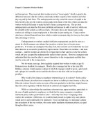
The market demand can be shown graphically as the horizontal summation of the
quantity of a product each individual will buy at each price. Assume that the market for
Coke is composed of two individuals, Anna and Betty, who differ in their demand for
Coke, as shown in Figure 8.2. The demand of Anna is D
A
and the demand of Betty is D
B
.
Then to determine the number of Cokes both of them will demand at any price, we
simply add together the quantities each will purchase, at each price (see Table 8.1). At a
price of $11, neither person is willing to buy any Coke; consequently, the market demand
must begin below $11. At $9, Anna is still unwilling to buy any Coke, but Betty will buy
two units. The market quantity demanded is therefore two. If the price falls to $5, Anna
wants two Cokes and Betty, given her greater demand, wants much more, six. The two
quantities combined equal eight. If we continue to drop the price and add the quantities
bought at each new price, we will obtain a series of market quantities demanded. When
plotted on a graph they will yield curve D
A+B
, the market demand for Coke (see Figure
8.2).

___________________________________

FIGURE 8.2 Market Demand Curve
The market demand curve for Coke, D

A+B
, is
obtained by summing the quantities that individuals
A and B are willing to buy at each and every price
(shown by the individual demand curves D
A
and
D
B
).







This is, of course, an extremely simple example, since only two individuals are
involved. The market demand curves for much larger groups of people, however, are
derived in essentially the same way. The demands of Fred, Marsha, Roberta, and others
would be added to those of Anna and Betty. As more people demand more Coke, the
market demand curve flattens out and extends further to the right.

Elasticity: Consumers’ Responsiveness to Price Changes
In the media and in general conversation, we often hear claims that a price change will
have no effect on purchases. Someone may predict that an increase in the price of
prescription drugs will not affect people’s use of them. The same remark is heard in
connection with many other goods and services, from gasoline and public parks to
medical services and salt. What people usually mean by such statements is that a price
Chapter 8 Consumer Choice and Demand in

Traditional and Network Markets



8
change will have only a slight effect on consumption. The law of demand states only that
a price change will have an inverse effect on the quantity of a good purchased. It does
not specify how much of an effect the price change will have.


TABLE 8.1 Market Demand for Coke

Quantity Quantity Quantity Demanded
Price Demanded by Demanded by by both Anna and Betty
of Coke Anna (D
A
) Betty (D
B
) (D
A+B
)
(1) (2) (3) (4)
$11 0 0 0
10 0 1 1.0
9 0 2 2.0
8 0.5 3 3.5
7 1.0 4 5.0
6 1.5 5 6.5
5 2.0 6 8.0
4 2.5 7 9.5

3 3.0 8 11.0
2 3.5 9 12.5
1 4.0 10 14.0


Note: The market demand curve, D
A+B
, in Figure 8.2 is obtained by plotting the quantities in column (4)
against their respective prices in column (1).

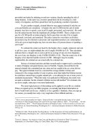
In other words, we have established only that the market demand curve for a
good will slope downward. The actual demand curve for a product may be relatively flat,
like curve D
1
in Figure 8.3, or relatively steep, like curve D
2
. Notice that at a price of P
1
,
the quantity of the good or service consumed is the same in both markets. If the price is
raised to P
2
, however, the response is substantially greater in market D
1
than in D
2
. In
D
1
, consumers will reduce their purchases all the way to Q

1
. In D
2
, consumption will
drop only to Q
2
.
Economists refer to this relative responsiveness of demand curves as the price
elasticity of demand. Price elasticity of demand is the responsiveness of consumers, in
terms of the quantity purchased, to a change in price, everything else held constant.
Demand is relatively elastic or inelastic, depending on the degree responsiveness to price
change. Elastic demand is a relatively sensitive consumer response to price changes. If
the price goes up or down, consumers will respond with a strong decrease or increase in
the quantity demanded. Demand curve D
1
in Figure 8.3 may be characterized as
relatively elastic. Inelastic demand is a relatively insensitive consumer response to price
changes. If the price goes up or down, consumers will respond with only a slight
decrease or increase in the quantity demanded. Demand curve D
2
in Figure 8.3 is
relatively inelastic.
The elasticity of demand is a useful concept, but our definition is imprecise.
What do we mean by “relatively sensitive” or “relatively insensitive”? Under what
Chapter 8 Consumer Choice and Demand in
Traditional and Network Markets



9

circumstances is consumer response sensitive or insensitive? There are two ways to add
precision to our definition. One is to calculate the effect of a change in price on total
consumer expenditures (which must equal producer revenues). The other is to develop
mathematically values for various levels of elasticity. We will deal with each in turn.



FIGURE 8.3 Elastic and Inelastic Demand
Demand curves differ in their relative elasticity.
Curve D
1
is more elastic than curve D
2
, in the sense
that consumers on curve D
1
are more responsive to
a price change than are consumers on curve D
2
.




Analyzing Total Consumer Expenditures
An increase in the price of a particular product can cause consumers to buy less.
Whether total consumer expenditures rise, fall, or stay the same, however, depends on the
extent of the consumer response. Many people assume that businesses will charge the
highest price possible to maximize profits. Although they sometimes do, high prices are
not always the best policy. For example, if a firm sells fifty units of a product for $1, its

total revenue (consumers’ total expenditures) for the product will be $50 (50 x $1). If it
raises the price to $1.50 and consumers cut back to forty units, its total revenue could
rise to $60 (40 x $1.50). If consumers are highly sensitive to price changes for this
particular good, however, the fifty-cent increase may lower the quantity sold to thirty
units. In that case total consumer expenditures would fall to $45 ($1.50 x 30).
1


1
To prove this result, let’s look at marginal revenue MR, or the change in total revenue in response to a
change in quantity Q. Taking the derivative of P(Q) • Q with respect to Q, we obtain
Q
dQ
dP
QP
dQ
QQPd
•+=
•
= )(
])([
MR
Factoring price out of the right-hand side of this equation gives us






•+=

P
Q
dQ
dP
P 1MR
which, because E =






−
dP
dQ
, is the same as
Chapter 8 Consumer Choice and Demand in
Traditional and Network Markets



10
The opposite can also happen. If a firm establishes a price of $1.50 and then
lowers it to $1, the quantity sold may rise, but the change in total consumer expenditures
will depend on the degree of consumer response. In other words, consumer
responsiveness determines whether a firm should raise or lower its price. (We will return
to this point later.)
We can define a simple rule of thumb for using total consumer expenditures to
analyze the elasticity of demand. Demand is elastic:
• if total consumer expenditures rise when the price falls, or

• if total consumer expenditures fall when the price rises.
Demand is inelastic:
• if total consumer expenditures rise when the price rises, or
• if total consumer expenditures fall when the price falls.

Determining Elasticity Coefficients
Although we have refined our definition of elasticity, it still does not allow us to
distinguish degrees of elasticity or inelasticity. Elasticity coefficients do just that. The
elasticity coefficient of demand (E
d
) is the ratio of the percentage change in the quantity
demanded to the percentage change in price. Expressed as a formula,
percentage change in quantity
E
d
= percentage change in price
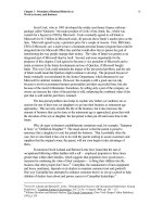
The elasticity coefficient will generally be different a different points on the
demand curve. Consider the linear demand curve in Figure 8.4. At every point on the
curve, a price reduction of $1 causes quantity demanded by rise by ten units, but a $1
decrease in price at the top of the curve is a much smaller percentage change than a $1
decrease at the bottom of the curve. Similarly, an increase of ten units in the quantity
demanded is a much larger percentage change when the quantity is low than when it is
high. Therefore the elasticity coefficient falls as consumers move down their demand
curve. Generally, a straight-line demand curve has an inelastic range at the bottom, a
unitary elastic point in the center, and an elastic range at the top.
2


1 if 0
1 if 0

1 if 0

1
1MR
<<
==
>>






−=
E
E
E
E
P
From this it follows immediately that an increase in Q (a decrease in P) increases total revenue if E > 1, has
no effect on total revenue if E = 1, and reduces total revenue if E < 1.
2
To prove this, we recognize that the equation for a linear domain curve can be expressed mathematically
as
Q
P
B
A
−
=

where P represents price, Q is quantity demanded, and A and B are positive constants. The total revenue
associated with this demand curve is given by
Chapter 8 Consumer Choice and Demand in
Traditional and Network Markets



11
___________________________________
FIGURE 8.4 Changes in the Elasticity Coefficient
The elasticity coefficient decreases as a firm moves
down the demand curve. The upper half of a linear
demand curve is elastic, meaning that the elasticity
coefficient is greater than one. The lower half is
inelastic, meaning that the elasticity coefficient is
less than one. This means that the middle of the
linear demand curve has an elasticity coefficient
equal to one.



There are two formulas for elasticity, one for use at specific points on the curve
and one for measuring average elasticity between two points, called arc elasticity. The
formula for point elasticity, which is used for very small changes in price, is:
change in quantity demanded change in price
E
d
= initial quantity demanded ÷ initial price
or

Q
1
- Q
2
P
1
- P
2

E
d
= Q
1
÷ P
1


The formula for arc elasticity is:



2
BA QQPQ −=
The marginal revenue is obtained by taking the derivative of total revenue with respect to Q or
Q
MR
B
2
A

−
=

From footnote 1, we know that when marginal revenue is equal to 0, elasticity is equal to 1. From Equation
(2) here, this implies that E = 1 when
0
B
2
A
=
−
Q

or when
B
A
2
1
•=Q
From Equation (1) we know that when the demand curve intersects the Q axis, P = 0 and
B
A
=Q
Thus, with a linear demand curve, E = 1 when Q is one-half the distance between Q = 0 and the Q that
drives price down to 0. The reader is invited to prove that E > 1 when Q < ½ • A/B, and that E < 1 when Q
> ½ • A/B.

Chapter 8 Consumer Choice and Demand in
Traditional and Network Markets

12
Q
1
Q
2
P
1
– P
2

E
d
= ½ (Q
1
+ Q
2
) ÷ ½ (P
1
P
2
)

Where the subscripts 1 and 2 represent two distinct points, or prices, on the demand
curve. Note that although the calculated elasticity is always negative, economists, by
convention, speak of it as a positive number. Economists, in effect, use the absolute
value of elasticity.
The change can be illustrated by computing the arc elasticity between two
sets of points, ab and cd. Arc elasticity between points a and because:

10 – 20 10 – 9 10 1 95
E
d
= ½ (10 + 20) ÷ ½ (10 + 9) = - 15 ÷ 9.5 = - 15 = -6.33
or 6.33 in absolute value.
Arc elasticity between points c and d:

90 – 100 2 – 1 10 1
E
d
= ½ (90 + 100) ÷ ½ (2 + 1) = -95 ÷ 1.5 = - 0.16 or 0.16 in absolute value.

Elasticity coefficients can tell us much at a glance. When the percentage
change in quantity is greater than the percentage change in price, an elasticity
coefficient that is greater than 1.0 results. In these cases, demand is said to be elastic.
When the percentage change in quantity is less than the percentage change in price,
the elasticity coefficient will be less than 1.0. Demand is said to be inelastic. When
the percentage change in the price is equal to the percentage change in quantity, the
elasticity coefficient is 1.0, and demand is unitary elastic.
3
In short:
Elastic demand: E
d
> 1
Inelastic demand: E
d
< 1
Unitary elastic demand: E

d
= 1
Elasticity coefficients enable economists to make accurate comparisons. A
demand with an elasticity coefficient of 1.75 is more elastic than one with an elasticity
coefficient of 1.55. A demand with a coefficient of 0.25 is more inelastic than one with a
coefficient of 0.78.
Although elasticity coefficients are useful for some purposes, their accuracy
depends on data that are often less than precise. In the real world, there is constant
change in the nonprice variables that influence how much of any product consumers
want. It is extremely difficult for economists to separate the effects of a change in price

3
Remember that all elasticity coefficients are negative and are preceded by a minus sign. (The demand
curve has a negative slope.) economists generally omit the minus sign, as we have seen.
Chapter 8 Consumer Choice and Demand in
Traditional and Network Markets



13
from all the other forces operating in the marketplace. Small differences in elasticity
coefficients may reflect the imperfections of statistical analysis rather than true
differences in consumer responsiveness to price.

Elasticity, Not the Same as Slope
Students often confuse the concept of elasticity of demand with the slope of the demand
curve. A comparison of their mathematical formulas, however, shows they are quite
different.

rise change in price

slope = run = change in quantity

percentage change in quantity
elasticity = percentage change in price

The confusion is understandable. The slope of a demand curve does say something
about consumer’s responsiveness: it shows how much the quantity consumed goes up
when the price goes down by a given amount. Slope is an unreliable indicator of
consumer responsiveness, however, because it varies with the units of measurement for
price and quantity. For example, suppose that when the price rises from $10 to $20,
quantity demanded decreases from 100 to 60. The slope is –1/4.

-10 -1
slope = 40 = 4

If a price is measured in pennies instead of dollars, however, the slope comes out to –25.

-1000 -25
slope = 40 = 1

No matter how the price is measured, the arc elasticity of demand remains –0.75.
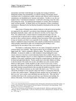
Furthermore, two parallel demand curves of identical slope will not have the same
elasticity coefficients. For example, consider the two curves in Figure 8.5. When the
price falls from $5 to $4, the quantity demanded rises by the same amount for each curve:
ten units. Yet the percentage change in quantity is substantially lower for D
2
than for D
1
.
(A rise from seventy to eighty is not nearly as dramatic in percentage terms as a rise from

twenty-five to thirty-five.) Thus the elasticity coefficient is lower for demand curve D
2
.
Be careful not to judge the elasticity of demand by looking at a curve’s slope.



Chapter 8 Consumer Choice and Demand in
Traditional and Network Markets



14
Applications of the Concept of Elasticity
Elasticity of demand is particularly important to producers. Together with the cost of
production, it determines the prices firms can charge for their products. We have seen
that an increase or decrease in price can cause total consumer expenditures to rise, fall, or
remain the same, depending on the elasticity of demand. Thus if a firm lowers its price
and incurs greater production costs (because it is producing and selling more units), it
may still increase its profits. As long as the demand curve is elastic, revenues can (but
will not necessarily) go up more than costs. Over the last three decades, the American
Telephone and Telegraph Company has frequently lowered its prices on long-distance
calls. To justify those decisions, AT&T had to reason that demand was sufficiently
elastic to produce revenues that would more than cover the cost of servicing the extra
calls. During the 1950s a 1960s, many electric power companies requested rate
reductions for the same reason.
Producers of concerts and dances estimate the elasticity of demand when they
establish the price of admission. If admission costs $10, tickets may be left unsold. At a
lower price, say $7, attendance and profits may be higher. Even if costs rise (for extra
workers and more programs), revenues can still rise more.

___________________________________
FIGURE 8.5 Two Parallel Curves Do Not Have
the Same Elasticity
Even two parallel demand curves of the same slope
do not have the same elasticity. Although a given
change in price—for example, a $1 change—will
produce the same unit change in quantity
demanded, the percentage change will differ.
Here, a drop in price from $5 to $4 produces a ten-
unit gain in quantity demanded on both curves
D
1
and D
2
. A ten-unit increase in sales represents a
lower percentage change at an initial sales level of
seventy (curve D
2
).
The difference in the elasticity of the two curves
can be illustrated by computing the arc elasticity
between two sets of points, ab on curve D
1
and cd
on curve D
2
. Arc elasticity between points a and b:
25 - 35 5 - 4
E
d

= ½(25 + 35) ÷ ½(5 + 4) = 1.50

Arc elasticity between points c and d:
70 - 80 5 - 4
E
d
= ½(70 + 80) ÷ ½(5 + 4) = 0.60


Government too must consider elasticity of demand, for the consumer’s demand
for taxable items is not inexhaustible. If a government raises excise taxes on cars or
jewelry too much, it may end up with lower tax revenues. The higher tax, added to the
final price of the product, may cause a negative consumer response. It is no accident that
Chapter 8 Consumer Choice and Demand in
Traditional and Network Markets



15
the heaviest excise taxes are usually imposed on goods for which the demand tends to be
inelastic, such as cigarettes and liquor.
The same reasoning applies to property taxes. Many large cities have tended to
underestimate the elasticity of demand for living space. Indeed, a major reason for the
recent migration from city to suburbs in many metropolitan areas has been the desire of
residents to escape rising tax rates. By moving just outside a city’s boundaries, people
can retain many of the benefits a city provides without actually paying for them. This
movement of city dwellers to the suburbs lowers the demand for property within the city,
undermining property values and destroying the city’s tax base. Thus, if governments
wish to maintain their tax revenues, they have to pay attention to the elasticity of demand
for living in their jurisdictions.

Determinants of the Price Elasticity of Demand
So far our analysis of elasticity has presumed that consumers are able to respond to a
price change. However, consumers’ ability to respond can be affected by various factors,
such as the number of substitutes and the amount of time consumers have to respond to a
change in price by shifting to other products or producers.

Substitutes
Substitutes allow consumers to respond to a price increase by switching to another good.
If the price of orange juice goes up, you are not required to go on buying it. You can
substitute a variety of other drinks, including water, wine, and soda.
The elasticity of demand for any good depends very much on what substitutes are
available. The existence of a large number and variety of substitutes means that demand
is likely to be elastic. That is, if people can switch easily to another product that will
yield approximately the same value, many will do so when faced with a price increase.
The similarity of substitutes—how well they can satisfy the same basic want—also
affects elasticity. The closer a substitute is to a product, the more elastic demand for the
product will be. If there are no close substitutes, demand will tend to be inelastic. What
we call necessities are often things that lack close substitutes.
Few goods have no substitutes at all. Because there are many substitutes for
orange juice—soda, wine, prune juice, and so on—we would expect the demand for
orange juice to be more elastic than the demand for salt, which has fewer viable
alternatives. Yet even salt has synthetic substitutes. Furthermore, though human beings
need a certain amount of salt to survive, most of us consume much more than the
minimum and can easily cutback if the price of salt rises. The extra flavor that salt adds
is a benefit that can be partially recouped by buying other things.
At the other extreme from goods with no substitutes are goods with perfect
substitutes. Perfect substitutes exist for goods produced by an individual firm engaged in
perfect competition. An individual wheat farmer, for example, is only one among
thousands of producers of essentially the same product. The wheat produced by others is

Chapter 8 Consumer Choice and Demand in
Traditional and Network Markets



16
a perfect substitute for the wheat produced by the single farmer. Perfect substitutability
can lead to perfect elasticity of demand.
The demand curve facing the perfect competitor is horizontal, like the one in
Figure 8.6. If the individual competitor raises his price even a minute percentage above
the going market price, consumers will switch to other sellers. The elasticity coefficient
of such a horizontal demand curve is infinite. Thus this demand curve is described as
perfectly elastic. A perfectly elastic demand is a demand that has an elasticity
coefficient of infinity. It is expressed graphically as a curve horizontal to the X-axis.

Time
Consumption requires time. Accordingly, a demand curve must describe some particular
time period. Over a very short period of time—say a day—the demand for a good may
not react immediately. It takes time to find substitutes. With enough time, however,
consumers will respond to a price increase. Thus a demand curve that covers a long
period will be more elastic than one for a short period.
___________________________________
FIGURE 8.6 Perfectly Elastic Demand
A firm that has many competitors may lose all its
sales if it increases its price even slightly. Its
customers can simply move to another producer.
In that case its demand curve is horizontal, with an
elasticity coefficient of infinity.

Oil provides a good example of how the elasticity of demand can change over
time. In 1973 Arab oil producers raised the price of their crude oil, and domestic oil
producers followed suit. For a time consumers were caught. Drivers were stuck with
big, gas-guzzling cars and with suburban homes located far from their work places.
Automakers were tooled up to produce big cars, not subcompacts. Over the long term,
however, alternative modes of transportation became available and alternative sources of
energy were found. People altered their lifestyles, walking or riding bicycles to work.
The long-term demand curve for oil is much more elastic than the short-term demand
curve.