Tài liệu Microeconomics for MBAs 28 doc

Chapter 8 Consumer Choice and Demand in
Traditional and Network Markets



17
Changes in Demand
The determinants of the elasticity of demand are fewer and easier to identify than the
determinants of demand itself. As we saw in Chapter 3, the demand for almost all goods
is affected in one way or another by (1) consumer incomes; (2) the prices of other goods;
(3) the number of consumers; (4) expectations concerning future prices and incomes; and
(5) that catchall variable, consumer tastes and preferences. Additional variables apply in
differing degrees to different goods. The amount of ice cream and the number of golf
balls bought both depend on the weather (very few golf balls are sold at the North Pole).
The number of cribs demanded depends on the birthrate. Together all these variables
determine the position of the demand curve. If any variable changes, so will the position
of the demand curve.
We saw in Chapter 3 that if consumer preference for a product—say, blue jeans—
increases, the change will be reflected in an outward movement of the demand curve (see
Figure 8.7). That is what happened during the late 1960s, when college students’ tastes
changed and wearing faded blue jeans became chic. By definition, such a change in taste
means that consumers are willing to buy more of the good at the going market price. If
the price is P
1
, the quantity demanded will increase from Q
2
to Q
3
. A change in tastes
can also mean that people are willing to buy more jeans at each and every price. At P
2

they are now willing to buy Q
2
instead of Q
1
blue jeans. We can infer from this pattern
that consumers are willing to pay a higher price for any given quantity. In Figure 8.7, the
increase in demand means that consumers are willing to pay as much as P
2
for Q
2
pairs of
jeans, whereas formerly they would pay only P
1
. (If consumers’ tastes change in the
opposite direction, the demand curve moves downward to the left, as in Figure 8.8, a
quantity demanded at a given price decreases.)
Whether demand increases or decreases, the demand curve will still slope
downward. Everything else held constant, people will buy more of the good at a lower
price than a higher one. To assume that other variables will remain constant, of course, is
unrealistic because markets are generally in a state of flux. In the real world, all variables
just do not stay put to allow the price of a good to change by itself. Even if conditions
change at the same time that price changes, the law of demand tells us that a decrease in
price will lead people to buy more than they would otherwise, and an increase in price
will lead them to buy less.
For example, in Figure 8.8, the demand for blue jeans has decreased, because
consumers are less willing to buy the product. A price reduction can partially offset the
decline in demand. If producers lower their price from P
2
to P

1
, quantity demanded will
fall only to Q
2
instead of Q
1
. Although consumers are buying fewer jeans than they once
did (Q
2
as opposed to Q
3
) because of changing tastes, the law of demand still holds.
Because of the price change, consumers have increased their consumption over what it
would otherwise have been.
A change in consumer incomes will affect demand in more complicated ways.
The demand for most goods, called normal goods, increases with income. A normal
good or service is any good or service for which demand rises with an increase in
income and falls with a decrease in income. The demand for a few luxury goods actually
outstrips increases in income. A luxury good or service is any good or service for which
Chapter 8 Consumer Choice and Demand in
Traditional and Network Markets



18
demand rises proportionally faster than income. An inferior good or service is any good
or service for which demand falls with an increase in income and rises with a decrease in
income. Beans are an example of a good many people would consider inferior. People
who rely on beans as a staple or filler food when their incomes are low may substitute
meat and other higher-priced foods when their incomes rise.

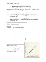
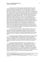
FIGURE 8.7 Increase in Demand
When consumer demand for blue jeans increases,
the demand curve shifts from D
1
to D
2
.
Consumers are now willing to buy a larger
quantity of jeans at the same price, or the same
quantity at a higher price. At price P
1
, for
instance, they will buy Q
3
instead of Q
2
. And

they are now willing to pay P
2
for Q
2
jeans,
whereas before they wold pay only P
1
.

_

___________________________________
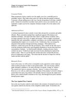
FIGURE 8.8 Decrease in Demand
A downward shift in demand, from D
1
to D
2
,
represents a decrease in the quantity of blue
jeans consumers are willing to buy at each and
every price. It also indicates a decrease in the
price they are willing to pay for each and every
quantity of jeans. At price P
2
, for instance,
consumers will now buy only Q
1
jeans (not Q
3
,

as before); and they will now pay only P
2
for Q
1

jeans not P
3
, as before.


Thus, while economists can confidently predict the directional movement of
consumption when prices change, they cannot say what will happen to the demand for a
particular good when income changes, because each individual determines whether a
particular good is a normal, inferior, or luxury good. Different people will tend to answer
this question differently in different markets. Beans may be an inferior good to most
low-income consumers and a normal good to many others.
For example, how do you think a change in income will affect the demand for
low-, medium-, and high-quality liquor? You may have some intuitive notion about the
effect, but you are probably not as confident about it as you are about the effect of a price
Chapter 8 Consumer Choice and Demand in
Traditional and Network Markets



19
decrease. In fact, during past recessions, the demand for both low- and high-quality
liquor has increased. Some consumers may have switched to high-quality liquor to
impress their friends, and to suggest that they have been unaffected by the economic
malaise. Others may have tried to maintain their old level of consumption by switching
to a low-quality brand.

The effect of a change in the price of other goods is similarly complicated. Here
the important factor is the relationship of one good—say, ice cream—to other
commodities. Are the goods in question substitutes for ice cream, like frozen yogurt?
Are they complements, like cones? Are they used independently of ice cream? Demand
for ice cream is unlikely to be affected by a drop in the price of baby rattles, but it may
well decline if the price of frozen yogurt drops.
Two products are generally considered substitutes if the demand for one goes up
when the price of the other rises. The price of a product does not have to rise above the
price of its substitute before the demand for the substitute is affected. Assume that the
price of sirloin steak is $6 per pound and the price of hamburger is $2 per pound. The
price difference reflects the fact that consumers believe the two meats are of different
quality. If the price of hamburger rises to $4 per pound while the price of sirloin remains
constant at $6, many buyers will increase their demand for steak. The perceived
difference in quality now outweighs the difference in price.
Because complementary products—razors and razor blades, oil and oil filters,
VCRs and videocassette tapes—are consumed jointly, a change in the price of one will
cause an increase or decrease in the demand for both products at once. An increase in the
price of razor blades, for instance, will induce some people to switch to electric razors,
causing a decrease in the quantity of razor blades demanded and a decrease in the
demand for safety razors. Again, economists cannot predict how many people will
decide the switch is worthwhile, they can merely predict from theory the direction in
which demand for the product will move.

Derivation of Demand from Indifference Curves
And the Budget Line
Our discussion of theoretical foundations of demand has, admittedly, been casual. Here
we can add greater precision to the analysis. Much of the discussion has been founded on
the notion of the rational pursuit of individual preferences. That is, we assume the
individual knows what he or she wants and will seek to accomplish those goals.
Preference, however, is a nebulous concept. To lend concreteness to the idea, economists

have developed the indifference curve.
Individuals face limits in what they can produce and buy, a point of earlier
chapters. That fact, together with the existence of indifference curves, can be used to
derive an individual’s demand for a product.



Chapter 8 Consumer Choice and Demand in
Traditional and Network Markets



20
Derivation of the Indifference Curve
Consider a student whose wants include only two goods, pens and books. Figure 8.9
shows all the possible combinations of pens and books she may choose. The student will
prefer a combination far from the origin to one closer in. At point b, for instance, she
will have more books and more pens than at point a. For the same reason, she will prefer
a to c. In fact the student will prefer a to any point in the lower left quadrant of the graph
and will prefer any point in the upper right quadrant to a.
We can also reason that the student would prefer a to d, where she gets the same
number of pens but fewer books than at a. Likewise, she will prefer e to a because it
yields the same number of books and more pens than a. If a is preferred to d and e is
preferred to a, then as the student moves from d to e, she must move from a less
preferable to a more preferable position with respect to a. At some point along that path,
the student will reach a combination of books and pens that equals the value of point a.
Assuming that combination is f (it can be any point between d and e), we can say that the
individual is indifferent between a and f.
Using a similar line of logic, we can locate another point along the line gih that
will be equal in value to a and therefore to f. In fact, any number of points in the lower

right-hand and upper left-hand quadrants of the graph are of equal value to a. Taken
together, these points form what is called an indifference curve (see curve I
1
in Figure
8.10).
_____________________________________
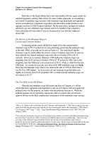
FIGURE 8.9 Derivation of an Indifference Curve
Because the consumer prefers more of a good to less,
point a is preferable to point c, and point b is
preferable to point a. If a is preferable to demand but
e is preferable to a, then when we move from point d
to e, we must move from a combination that is less
preferred the one that is more preferred. In doing so
we must cross a point—for example, f—that is equal
in value to a. Indifference curves are composed by
connecting all those points—a, f, i, and so on—that
are of equal value to the consumer.




Using a similar line of logic, we can locate another point along the line gih that
will be equal in value to a and therefore to f. In fact, any number of points in the lower
right-hand and upper left-hand quadrants of the graph are of equal value to a. Taken
together, these points form what is called an indifference curve (see curve I
1
in Figure
8.10). An indifference curve shows the various combinations of two goods that yield
the same level of total utility.
Chapter 8 Consumer Choice and Demand in

Traditional and Network Markets



21
Using the same line of reasoning, we can construct a second indifference curve
through point b. Because b is preferable to a, and all points on the new indifference
curve will be equal in value to point b, we can conclude that any point along the new
curve I
2
is preferable to any point on I
1
. Using this same procedure, we can continue to
derive any number of curves, each one higher than, and preferable to, the last.
From this line of reasoning, an economist can draw several conclusions about the
student’s preference structure (called an “indifference map”):
1. The student’s total utility level rises as she moves up and to the right, from one
indifference curve to the next.
2. Indifference curves slope downward to the right.
3. Indifference curves cannot intersect. (An intersection would imply that all points
on all the intersecting curves are of equal value, contradicting the conclusion that
higher indifference curves represent higher levels of utility).



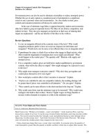
FIGURE 8.10 Indifference Curves for
Pens and Books
Any combination of pens and books that falls along
curve I
1

will yield the same level of utility as any
other combination on that curve. The consumer is
indifferent among them. By extension, any
combination on curve I
2
will be preferable to any
combination on curve I
1
.





The Budget Line and Consumer Equilibrium
From indifference curves we can derive the law of demand. First we need to construct
the individual’s budget line, a special form of the production possibilities curve. The
budget line shows graphically all the combinations of two goods that a consumer can buy
with a given amount of income. Assume that our student earns an income of $150, which
she uses to buy books and pens. Books cost $3 each and pens cost $5 a package. The
student can spend all $150 on fifty books or thirty pen packs, or she can divide her
expenditures in any number of ways to yield various combinations of books and pens.
By plotting all the possible combinations, we obtain the student’s budget line, B
1
P
1
in
Figure 8.11.
All combinations on the budget line are possible for the student. She can choose
point a, twenty-five books and fifteen pen packs, or point b, forty-five books and three

Chapter 8 Consumer Choice and Demand in
Traditional and Network Markets



22
pen packs. Either combination exhausts her $150 budget. The rational individual will
choose that point where the budget line just touches (is tangent to) an indifference
curve—point a in this case.
4
Points farther up or down the budget line will put the
student on a lower indifference curve and are therefore less preferable. (If, for instance,
the student moves to c on the budget line, she will be on a lower indifference curve, I
2

instead of I
1
.) At point a, the individual’s wants are said to be in equilibrium. As long as
her income and preferences and the prices of books and pens remain the same, she has no
reason to move from that point.
5


4
This tangency condition can be derived mathematically by maximizing the consumer's utility subject to
the budget constraint, or by maximizing the U (X,Y) with respect to X and Y, subject to P
x
X + P
y
Y = I.

This constrained maximization problem can be carried out by forming the Lagrangian function
)()(
1
YPXPIYXUL
YX
−−+= λ
where λ is known as a Lagrangian multiplier, and maximizing it with respect to X and Y and minimizing it
with respect to λ. The necessary conditions are
0=−
∂
∂
=
∂
∂
X
P
X
U
X
L
λ

0=−
∂
∂
=
∂
∂
Y
P

Y
U
Y
L
λ

0=−−=
∂
∂
YPXPI
L
YX
λ

Equation (1) can be divided by equation (2), which, after simple algebraic manipulation, yields

(Missing equation to be added).

The left-hand side of this equation is -1 multiplied by the ratio of the marginal utility of good X to the
marginal utility of good Y, or the slope of the indifference curve. The right-hand side is -1 multiplied by
the ratio of the price of good X to the price of good Y, or the slope of the budget constraint.
The equality of these two slopes is dependent on the assumption that the consumer will consume
positive quantities of both goods. Later in this chapter, we will consider the possibility that the consumer
may maximize utility subject to the budget constraint by deciding to consume none of one of the goods.

5
We can provide another intuitive rationale for the required condition for consumer equilibrium. Starting
with the tangency requirement
Y
X

Y
X
P
P
MU
MU
=
we can obtain the equivalent condition
Y
Y
X
X
P
MU
P
MU
=
by simple algebraic manipulation. Verbally, this means that the consumer receives the same increase in
utility from spending $1 more on good X as would be received from spending more on good Y. We can
see that this condition is necessary if utility is being maximized subject to the budget constraint by
assuming that the condition is not satisfied. Assume for example, that (continued on next page)
Y
Y
X
X
P
MU
P
MU
>

Chapter 8 Consumer Choice and Demand in
Traditional and Network Markets



23
___________________________________
FIGURE 8.11 The Budget Line and Consumer
Equilibrium
Constrained by her budget, the consumer will
seek to maximize her utility by consuming at the
point where her budget line is tangent to an
indifference curve. Here the consumer chooses
point a, where her budget line just touches
indifference curve I
1
. All other combinations on
the consumer’s budget line will fall on a lower
indifference curve, providing less utility. Point c,
for instance, falls on indifference curve I
2
.
_________________________________




What happens if prices change? Suppose the individual’s wants are in
equilibrium at point a in Figure 8.11 when the price of pens falls from $5 a pack to $3 a
pack. (The price of books stays the same.) The budget line will pivot to B

1
P
2
in Figure
8.12, reflecting the greater buying power of the student’s income. (She can now buy fifty
pen packs with $150.) The new budget line gives the student a chance to move to a
higher indifference curve—for instance, to point c, twenty-two pens and twenty-eight
books.

The Law of Demand, Again
The result of the price reduction is that the student buys more pens. Thus we derive the
law of demand, that quantity demanded is inversely related to price. The downward-
sloping demand curve for pens shown in Figure 8.13 is obtained by plotting the quantities
of pen packs bought from Figure 8.12 against the price paid per pack. When the price of
pens falls from $5 to $3 a pack in Figure 8.12, the consumer increases the quantity
purchased from fifteen to twenty-two packages.


This tells us that if $1 less is spent on good Y, utility will not decline as much as it will increase if $1 more
is spent on good X. Therefore, the consumer can increase total utility without increasing expenditures by
reducing the consumption of good Y and increasing the consumption of good X. This will continue to be
true until the equality is restored, which will happen eventually as MU
Y
increases relative to MU
X
. In a
similar manner, we can argue that the consumer will move toward the equilibrium condition if we assume
that
Y
Y

X
X
P
MU
P
MU
<

Chapter 8 Consumer Choice and Demand in
Traditional and Network Markets



24












FIGURE 8.12 Effect of a change in Price on
Consumer Equilibrium
If the price of pens falls, the consumer’s budget
line will pivot outward, from B

1
P
1
to B
1
P
2
. As a
result, the consumers can move to a higher
indifference curve, I
2
instead of I
1
. At the new
price the consumer buys more pens, twenty-two
packs as opposed to fifteen.


FIGURE 8.13 Derivation of the Demand Curve
for Pens
When the price of pens changes, shifting the
consumer’s budget line from I
1
to I
2
in Figure 8.14, the
consumer equilibrium point changes with it. The
consumer’s demand curve for pens is obtained by
plotting her equilibrium quantity of pens at various
prices. At $5 a pack, the consumer buys fifteen packs

of pens (point a). At $3 a pack, she buys twenty-two
packages (point c).

Application: Cash Versus In-Kind Transfers
A cash grant will raise the welfare of the poor more than an in-kind transfer of equal
value. Figure 8.14 illustrates a poor family’s budget line for higher education and
housing, H
3
E
3
. Without subsidies, this family can buy as much as E
3
units of education
(and no housing) or H
3
units of housing (and no education). Because the family wants
both housing and higher education, it will probably divide its income between the two,
choosing some combination like point a, or E
1
education and H
1
housing.
Suppose that the government decides to subsidize the family’s higher education
purchases through reduced university tuition. Its action lowers the total price of
education, pivoting the family’s budget line out to H
3
E
5
. The result is that the family can
now consume more of both items, education and housing. The family will probably

move to some combination like b, H
2
housing and D
2
education Its education
consumption has gone up and the additional housing purchased represents an increase in
income equal to the vertical distance between b and c.
Suppose the family were given the cash equivalent of bc instead. The additional
money would not change the relative prices of higher education and housing, as the
reduced tuition program did. It would shift the budget line from H
3
E
3
to a parallel
position, H
4
E
4
(dashed line). The relative price of housing is lower on H
4
E
4
than on

Chapter 8 Consumer Choice and Demand in
Traditional and Network Markets

25

25

H
3
E
5
. Thus the family would tend to prefer d to b, both of which are available on line
H
4
E
4
, we must presume that they would prefer cash to an in-kind subsidy.
This point can be seen even more clearly with the help of indifference curves.
Imagine an indifference curve tangent to H
3
E
3
in the absence of government relief,
causing the family to point a. Imagine a higher indifference curve that is tangent to H
3
E
5

at point b. Now, imagine an even higher indifference curve tangent to H
4
E
4
at point d.


__________________________________________
FIGURE 8.14 Budget Line: Cash Grants versus

Food Stamps
If the price of education is reduced by an in-kind
subsidy, a family’s budget line will pivot from
H
3
E
3
to H
3
E
5
. The family will move from point a
to point b, where it can consume more food and
housing. If the family is given the same subsidy in
cash, its budget line will move from H
3
E
3
to H
4
E
4
.
Since the relative price of housing is lower on H
4
E
4

than on H
3

E
5
, the family will choose a point like d
over b. Since b was the family’s preferred point on
H
3
E
5
, but they prefer d to b, we must presume they
also prefer cash to a food subsidy.
_________________________________________




Application: Capturing the Consumer surplus
The price that a consumer pays for a good reflects the value that he or she places on an
additional unit of the good. Since the price normally applies uniformly to all units of the
good purchased and the consumer generally values the last unit consumed less than the
units consumed previously, the consumer values the total consumption of a good at more
than the amount paid for its consumption. The gap between what a consumer is willing
to pay rather than do without a good (the total value placed on the good) and what the
consumer actually pays is referred to as the consumer surplus. Obviously, suppliers
prefer that consumers pay more rather than less for a good and are anxious to capture as
much consumer surplus as possible. We can employ indifference-curve analysis to show
how suppliers use different pricing schemes to encourage consumers to pay more for a
given quantity of a good than they would if the good were uniformly priced.
Conceptually, the simplest way for a supplier to capture the total consumer
surplus of an individual would be to charge a different price for each unit consumed and
to price each unit at the maximum amount the consumer is willing to pay for that unit.

But such a pricing policy would be enormously difficult to implement. The supplier
Chapter 8 Consumer Choice and Demand in
Traditional and Network Markets

26

26
would have to obtain detailed information about all consumers' preferences. Also,
consumers who place a relatively small value on the good and therefore purchase it for
less, would have to be prevented from selling the good to consumers who value it more
highly. Otherwise, low-demand consumers would be able to buy the good at a relatively
cheap price and profitably undercut the price that the supplier is charging the high-
demand consumers.
A final and related difficulty is that the more competitors a supplier has, the more
difficult it is to charge the same customer different prices for different units or to charge
different customers different prices. Although a consumer may be willing to pay the only
supplier of a good more for the first unit than the second unit, more for the second unit
than the third unit, and so on, this is not necessarily true when the consumer can choose
among several suppliers. A consumer will not be willing to pay one supplier any more
for a particular unit of a good than is being charged by an alternative supplier. The
consumer still values the first unit of the good more than the second unit, but competition
among several suppliers makes it difficult for any one supplier to take advantage of this
fact by imposing a different pricing strategy on each consumer and charging each
consumer a different price for each unit purchased. However, relatively crude or simple
price-discrimination schemes can be implemented that allow suppliers to capture more of
the consumer surplus than they could under a uniform pricing policy.
Such a price-discrimination scheme is illustrated in Figure 8.15 with the aid of an
individual's indifference-curve map. We assume the individual is initially at
Y
,

consuming
Y
units of good Y and no units of good X. Indifference curve I
1
indicates the
consumer's level of satisfaction for this consumption bundle. Given an opportunity to
purchase good X at a uniform price, reflected in the slope of budget constraint YX , the
consumer will purchase X
2
units and increase satisfaction by reaching the higher
indifference curve I
2
. Increased satisfaction is derived because less is being paid for the
X
2
units than they are worth to the consumer. The total value of the X
2
units to the
consumer is given in Figure 8.15 by the distance
1
YY− , which is the maximum amount
of good Y the consumer is willing to sacrifice to obtain X
2
units. (The consumer is
indifferent between
Y
units of Y and no X and Y
1
units of Y and X
2

units of X.) But
given the budget constraint YX , the consumer only has to sacrifice
2
YY− units of Y to
obtain X
2
units of X. The distance Y
2
– Y
1
measures the consumer surplus associated
with the consumer's ability to buy good X at a uniform price.
The supplier is interested in whether a relatively simple pricing strategy will
capture some of this consumer surplus. The supplier's objective is to raise the price and
still have the consumer purchase the same quantity of good X. If the supplier raises the
price uniformly, however, the budget constraint will pivot to the left around point
Y
, and
the consumer can be expected to purchase fewer units of good X. But what will happen
if the supplier imposes a two-part pricing policy, which allows the consumer to
purchase good X at a lower price if a specified number of initial units of X are purchased
at a higher price? Assume, for example, that the consumer faces the budget constraint
XaY in Figure 8.15. If the first X
1
units of good X are purchased at the higher price