Tài liệu Microeconomics for MBAs 30 pptx

Chapter 8 Consumer Choice and Demand in
Traditional and Network Markets

37

37
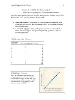
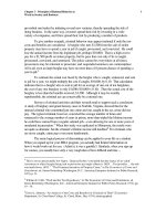
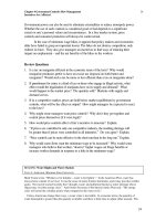
curves (the dark lines) are each very inelastic, but the long-term demand curve (dashed
line) is rather elastic. Indeed, Becker and Murphy maintain that the more addictive the
good, the more elastic will be the long-term demand.
13
This is the case because a
reduction in the current time period might not stimulate current sales very much.
However, for highly addictive goods, current consumption can give an even greater
increase in the future demand because the buyers “have to have more of it bad,” thus
resulting in even more future consumption than would be the case for less addictive
goods. Hence, it is altogether understandable why cigarette firms decades ago would
often have “cigarette girls” parading around campus in short skirts giving away small
packs of cigarettes and why many drug dealers to this day eagerly give away the first
“hits” to their potential customers. Indeed, it seems reasonable to conclude from the
Becker/Murphy line of argument, the more addictive the good, the lower the current
price. We might not even be surprised that for some highly addictive goods, the
producers would “sell” their goods at below zero prices (or would pay their customers to
take the good).

_____________________________
FIGURE 8.20 The Lagged Demand
Curve
As the price falls from P
3
to P
2

, the
quantity demanded in the short run rises
from Q
1
to Q
2
. However, sales build on
the sales, causing the demand in the
future to expand outward to, say, D
2
.
The lower the price in the current time
period, the greater the expansion of
demand in the future. The more the
demand expands over time in response to
greater sales in the current time period,
the more elastic in the long-run demand.
___________________________

In contrast to the theory of lagged demand, this theory of rational addiction
suggests explanations for a variety of behaviors, most notably, the observed differences
in the consumption behavior of young and old, the tendency of overweight people to go
on “crash diets” even when they may only want to lose a modest amount of weight, or
alcoholics who become “teetotalers” when they decide to curtail their drinking. Old
people may be less concerned about addictive behavior, everything else held constant,
than the young. Old people simply have less to lose over time from addictions than
younger people (given their shorter life expectancies). People who are addicted to food

13
Becker and Murphy conclude, “Permanent changes in prices of addictive goods may have a modest

short-run effect on the consumption of addictive goods. This could be the source of a general perception
that addicts do not respond much to changes in price. However, we show that the long-run demand for
addictive goods tends to be more elastic than the demand for nonaddictive goods” (Ibid, p. 695).
Chapter 8 Consumer Choice and Demand in
Traditional and Network Markets

38

38
may rationally choose to drastically reduce their intake of food even though they may
need to lose only a few pounds because their intake of food compels them to “over-
consume.” Similarly, alcoholics may “get on the wagon” in order to temper their future
demands for booze because even a modest consumption level can have a snowballing
effect, with a little consumption leading to more drinks, which can lead to even more.
Standard excise-tax theory suggests that producers’ opposition to excise taxes
should be tempered by the fact that the tax can be extensively passed onto the consumers
in the form of a price increase (that must always be less than the tax itself). The theory of
lagged demand suggests otherwise: producers of such goods have a substantial incentive
to oppose the tax because of the elastic nature of their long-run demands. While they
may be able to pass along a major share of the tax in the short run, they will not be able to
do so in the long run.

Lagged Demands, Rational Addiction,
And Excise Taxes
As we showed early in this book, an excise tax imposed on the production of a
good can be expected to have several effects.
• First, the supply of the good will be curbed.
• Second, the price consumers pay will rise with the curtailment in supply.
• Third, the price received by producers after the tax will fall.
The difference between the price paid by consumers and price received by the producers

equals the excise tax. (See Chapter 5 for a graphical presentation of these points.)
As you might imagine, the consequences of an excise tax for a good subject to a
lagged demand or rational addiction are not exactly the same. The excise tax might
indeed decrease the supply curve, as is the case of the standard good covered in Chapter
5. However, the impact on price and quantity sold will not likely be the same. This is
because of the incentive the producers have to suppress the current price to stimulate
future demand. When the prospects of the excise tax being enacted are evident to
producers, they can be expected to raise their prices currently (before the tax is enacted).
This means that the prospects of an excise tax can lead to a higher current price being
received by producers, as well as a lower quantity sold (even without the excise tax in
effect). When the tax is imposed, the reduction in quantity sold can be from two forces.
First, the price increase caused by the excise tax. Second, the price increase caused by
the prospects of the tax and the fact that the tax might be raised in the future.

Network Externalities
The theory of “network effects” or “network externalities” shares one key
construct with the theory of lagged demand and rational addiction: the interconnectedness
of demands. The interconnectedness in the theory of lagged demand and rational
addiction is through time. The interconnectedness in the theory of network effects and
externalities is across people and markets. The theory of network effects and
Chapter 8 Consumer Choice and Demand in
Traditional and Network Markets

39

39
externalities is best understood in terms of telephone systems that actually form
“networks,” that is, are tied together with telephone lines (as well as microwave disks and
satellites). No one would want to own a phone or buy telephone service if he or she were
the only phone owner. There would be no one to call. However, if two people – A and B

buy phones then each person has someone to call, and there are two pair-wise calls that
can be made: A can call B, and B can also call A. As more and more people buy phones,
the benefits of phone ownership escalate geometrically, given that there are progressively
more people to call and even more possible pair-wise calls. If there are three phone
owners – A, B, and C – then calls can be made in six pair-wise ways: A can call B or C,
B can call A or C, and C can call A or B. If there are four phone owners, then there are
12 potential pair-wise calls; five phone owners, 20 potential pair-wise calls; 20 phone
owners, 380, and so forth. If the network allows for conference calls, the count of the
ways calls can be made quickly goes through the roof with the rise in the number of
phone owners. It’s important to remember that the benefits buyers garner from others
joining the network can rise just from the potential to call others; they need not ever call
all of the additional joiners. Neither of the authors ever expects to call every business in
the country, but each author still gains from having the opportunity to call any of the
businesses that have phones.
Accordingly, the demand for phones can be expected to rise with phone
ownership. That is to say, the benefits from ownership go up as more people join the
network. Hence, people should be willing to pay more for phones as the count of phone
owners goes up. Some of the benefits of phone ownership are said to be “external” to the
buyers of phones because people other than those who buy phones gain by the purchases
(as was true in our study of public goods and external benefits studied in the last chapter).
In more concrete terms, when one of the authors, Lee, buys a phone, then the other
author, McKenzie, gains from Lee’s purchase and McKenzie pays nothing for Lee’s
phone. For that matter, everyone who has a phone gains more opportunities to call as
other people buy phones, or as the network expands (at least up to some point). The
gains that others receive from Lee’s or anyone else’s purchase are “external” to Lee,
hence are dubbed “external benefits” or, more to the point of this discussion, “network
externalities.”
In passing, we note that networks and network goods tend to turn one basic
economic proposition on its head. There is a canon in economic theory that we have
stressed from the start: As any good becomes scarcer, it becomes more valuable. In the

case of network goods, just the opposite is true: as the good become more abundant, its
value goes up.
14

There are two basic problems that a phone company faces in building its network.
First, the company has the initial problem of getting people to buy phones, given that at
the start the benefits will be low. Second, if some of the benefits of buying a phone are
“external” to the buyer, then each buyer’s willingness to buy a phone can be impaired.
How does the phone company build the network? One obvious solution is for the phone
company to do what the producers in the theory of lagged demand and rational addiction

14
See Kevin Kelly, New Rules for the New Economy (New York: Viking/Penguin Group, 1998), chap. 3.

Chapter 8 Consumer Choice and Demand in
Traditional and Network Markets

40

40
do: “under price” (or subsidize) their products – phones or, at the extreme, give them
away (or even pay people to install phones in their houses and offices).

Software Networks
The network effects in the software industry – for example, operating systems
are similar but, of course, differ in detail from the network effects in the telephone
industry. Indeed, the software developer may face more difficult problems, given that the
software development must somehow get the computer users on one side of the market
and application developers on the other side to join the network more or less together.
Few people, other than “geeks,” are likely to buy an operating system without

applications (for example, word processing programs or games) being available. If a
producer of an operating system is only able to get a few consumers to buy and use its
product, the demand for the operating system can be highly restricted. This will be the
case because few firms producing applications will write for an operating system with a
very limited number of users, given the prospects of few sales for their applications.
However, the applications written for the operating system can be expected to grow with
the number of people using the system. Why? Because the potential sales for
applications will grow with the expansion in the installed base of computers using the
operating system. If more applications are written for the operating system, then more
people will want to buy and use the operating system – which can lead to a snowball
effect: more sales, more applications, and even more sales in an ever expanding array of
people connected to the operating system by way of the invisible “network.”
As in the case of telephones, some of the benefits of purchases of the operating
system (and applications) are “external” to the people who buy them. People who join
the operating system network increase the benefits of all previous joiners, given that they
have more people with whom they can share computers or share data and manuscripts.
All joiners have the additional benefit of knowing that a greater number of operating
system users can increase the likelihood of more applications from which they can
choose. However, as in phone purchases, when the benefits are “external,” potential
users have an impaired demand for buying into the network. The greater the “external
benefits,” the greater buying resistance (or willingness to cover the operating system
cost).
The network may grow slowly at the start, because people (both computer users
and programmers) might be initially skeptical that any given operating system will be
able to become a sizable network (and provide the “external benefits” that a large
network can provide). However, as in the case of phones, “abundance” (not scarcity) can
imply greater value for the software/operating system network.
As the network for a given operating system grows, more and more people will
begin to believe that the operating system will become sizable, if not “dominant,” which
means that the network can grow at an escalating pace. As the network grows, there can

be some “tipping point,” beyond which the growth in the market for the operating system
will take on a life of its own, that is, grow at an ever faster pace because it has grown at
an ever faster pace. People will buy the operating system because everyone else is using
Chapter 8 Consumer Choice and Demand in
Traditional and Network Markets

41

41
it (which can mean, it needs to be stressed, that the self-accelerating growth in buyers of
one operating system can translate into the contraction of the market share for other
operating systems). After the “tipping point” has been reached, the firm’s eventual
market dominance – and monopoly power is practically assured, according to the
Justice Department.
This discussion might have relevance to the history of the dominance of the Apple
and Microsoft operating systems. Before the introduction of the IBM personal computer,
Apple was the dominant personal computer, running the CP/M operating system.
15

However, IBM and Microsoft developed their respective operating systems, PC-DOS and
MS-DOS, in 1981. At that time, ninety percent of programs ran under some version of
CP/M.
16
CP/M’s market dominance was likely undermined by two important factors:
First, CP/M was selling at the time for $240 a copy; DOS was introduced at $40.
17

Second, the dominance of IBM in the mainframe computer market could have indicated
to many buyers that some version of DOS would eventually be the dominant operating
system. In addition, Apple refused to “unbundle” its computer system: it insisted on

selling its own operating system with the Macintosh (and later generation models), and at
a price inflated by the restricted availability of Apple machines and operating systems.
Microsoft took a radically different approach: It got IBM to agree to allow it to
license MS-DOS to other manufacturers and then did just that to all comers, presumably
in the expectation that the competition among computer manufacturers on price and other
attributes of personal computers would spread the use of computers – and, not
incidentally, Microsoft’s operating system. The expected “abundance” of MS-DOS
systems led to an even greater demand for such systems, and to a lower demand for
Apple systems. Many people started joining the Microsoft network, presumably, not
always because they thought MS-DOS or Windows was a superior operating system to
Apple’s, but because any inferiority in the technical capabilities (if that were the case)
would be offset by the benefits of the greater size network. Supposedly, as the network
story might be told, there was a “tipping point” for Microsoft sometime in the late 1980s
or early 1990s (possibly with the release of Windows 3.1) that caused Windows to take
off, sending Apple into a market-share tailspin.
In 1998, the Justice Department took Microsoft to court for violation of the
nation’s antitrust laws. Among other charges, the Justice Department maintained that
Microsoft was a monopolist, as evidenced by its dominant (90+ percent) market share in
the operating system market, and that Microsoft was engaging in “predatory” pricing of
its browser Internet Explorer. Microsoft had been giving away Internet Explorer with
Windows 95 and had integrated Internet Explorer into Windows 98. The Justice
Department claimed that the only reason Microsoft could possibly have had to offer
Internet Explorer is to eliminate Netscape Navigator from the market. We can’t settle

15
David S. Evans, Albert Nichols, and Bernard Reddy, “The Rise and Fall of Leaders in Personal
Computer Software,” (Cambridge, Mass.: National Economic Research Associates, January 7, 1999), p. 4.

16
Ibid.

17
Ibid.

Chapter 8 Consumer Choice and Demand in
Traditional and Network Markets

42

42
these issues here. All we can actually do is point out that the Justice Department starts its
case against Microsoft with the claim that software markets are full of “network effects.”
While it might be true that Microsoft may have been engaging in predatory pricing, all
we can say here is that it may also be true that Microsoft was responding to the dictates of
“network effects,” underpricing its product in order to build its network and future
demand. It had another reason to lower its price to levels that Netscape might not
consider reasonable. If Microsoft lowers its price on Internet Explorer (or lowered its
effective price for Windows by including Internet explorer in Windows), then more
computers could be sold, which means more copies of Windows would be sold and more
copies of Microsoft’s applications – Word, Excel, etc. – would be sold. This means that a
lower price for Internet Explorer or Windows could give rise to higher sales, prices, and
profits on the applications.

MANAGER’S CORNER: Covering Relocation
Costs of New Hires
Major corporations are constantly hiring workers from one part of the country
only to ask them to move to another part, often a more expensive part. They also often
ask their employees to relocate, moving them from one location with a low cost of living
to another location with a higher cost of living. Few question whether the firms ordering
the movement should pay the cost of the moving van and travel. The trickier issue is

whether companies need to fully cover the difference in the cost of living.
As you can imagine, our best answer is that “it depends.” But we can do better
than that. We can show that if the cost-of-living difference is spread across all goods
bought by the relocating workers, the living cost difference will likely have to be
covered. However, if the cost difference is concentrated in any one good, for example,
housing, the firm can get by with increasing the relocating workers’ salaries by less than
the cost-of-living difference.
To see these points, which allow us to deduce general principles, suppose that
your company’s headquarters is in La Jolla, California, where the cost of housing is much
higher than in many other parts of the country. Suppose also that you want to hire an
engineer from Six Mile, South Carolina where the cost of housing is relatively low. In
fact, suppose you learn that the cost of housing in La Jolla is exactly five times the cost of
housing in Six Mile. A modestly equipped 2,000 square foot house in La Jolla on a one-
tenth of an acre lot, for example, sells for about $500,000. Approximately the same
house can be bought in Six Mile (with much more land) for $100,000.
The engineer you are interested in hiring is earning $100,000 a year in Six Mile.
In your interviews with the engineer, she tells you, quite honestly, that she likes the job
you have for her. However, she also informs you that after comparing La Jolla with her
hometown she has found that housing is the only major cost difference. That is, there are
minor cost differences for things like food, clothing, and medical care, but those
differences wash out, especially after considering quality differences. The two areas are
substantially different, she admits, but she values the amenities in the two locations more
or less the same. La Jolla has the ocean close by, but Six Mile has the mountains just a
short distance to the west.
Chapter 8 Consumer Choice and Demand in
Traditional and Network Markets

43

43

However, the engineer stresses that at an interest rate of 8.5 percent, the $400,000
additional mortgage she will have to take out to buy a house in La Jolla that is
comparable to the one she has back in Six Mile means an added annual housing
expenditure for her of $34,000. Therefore, she wants you to compensate her for the
difference in the cost of housing, which implies an annual salary of $134,000 (plus she
expects all moving and adjustment costs to be covered by your firm).
Do you have to concede to her demands? Many managers do succumb to the
temptation to concede to such demands. But, assuming that she is being truthful when
she says that the amenities of the areas and the other costs of living balance out, the
answer is emphatically, No. You should be able to get by with paying her something less
than $134,000 a year. There are two ways of explaining the “no” answer. First, you
should recognize that the engineer is getting a lot of purchasing power back in Six Mile
in one good, housing. If you gave her the demanded $34,000 in additional salary, she
would be able to replace her Six Mile house in La Jolla. However the money payment
you provide is fungible, which means that she could buy any number of other things with
the added income, including more time at the beach (than she spent in the mountains back
in Six Mile) or more meals out (and there are far more restaurants in La Jolla).
Hence, the engineer would actually prefer the $134,000 annual income in La Jolla
than the $100,000 income in Six Mile, which goes a long way toward explaining why she
is pressing the issue. If that is the case, she could also be happier in La Jolla with
something less than $134,000 in salary than she is in Six Mile. To get her to take your
job, all you need to do is make her slightly better off at your company’s location than she
is in Six Mile. Doing that does not require full compensation in the housing cost.
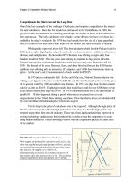
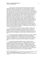
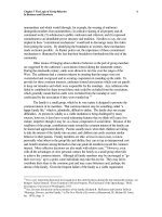
Another way of making the same point, but with greater clarity, is through the use
of Figure 8.21, which contains a representation of the engineer’s income constraints (or
“budget lines” for those who remember their formal economics training) in the two
locations. To make the analysis as simple as possible, and stay within the constraints of
the two-dimensional graph, we consider two categories of goods: housing, which is on
the horizontal axis, and a representative bundle of all other goods on the vertical axis.
The figure shows that with her $100,000 salary in Six Mile, the engineer can buy

H
1
units of housing, if she spent all of her income on housing (which, admittedly, would
never be practical), or she could buy A
1
bundles of all other goods, if she bought no
housing (which is also not practical). More than likely, the engineer will buy some
combination of housing and all other goods, say, combination a, H
2
of housing and A
2
of
all other goods.
If the engineer were only to get the same $100,000 in income in La Jolla, she
would have to choose from the combinations along the inside curve, which extends from
A
1
(meaning she could still buy, at the limit, the same number of bundles of all other
goods) to H
3
(much less housing if only housing were bought). Clearly, the engineer
would be unlikely to take an offer of $100,000, simply because there is no combination
along A
1
H
3
that is superior to combination a in Six Mile.
Chapter 8 Consumer Choice and Demand in
Traditional and Network Markets

44

44
If you conceded to her demand of $134,000 in annual income, her income
constraint would be the thin line that is parallel to A
1
H
3
and goes through a.
18
Clearly, she
could be as well off in La Jolla at such a salary because she could still take combination
a, but is she likely to do that?
















FIGURE 8.21 Choosing between Housing and Bundles of Other Goods

The budget line in Six Mile is A
1
H
1
with an income of $100,000. The budget
line in L Jolla is A
1
H
3
with the same income. If the employer were to offer the
engineer a salary of $134,000, which cover the additional cost of housing, the
engineers budget line would be the thin line cutting A
1
H
1
at a. Hence, the
engineer could choose combination b and be better off than in Six Mile. This
means that the employer can offer the engineer less than $134,000.
_______________________________________________________________

The answer is not likely, because of the changes in relative prices. The price of
housing in La Jolla is much higher than the price of housing in Six Mile, which is why
her dashed income constraint is much steeper than her old income constraint (A
1
H
1
).

18
By giving the engineer $134,000, she can buy the exact combination of goods that she had back in Six

Mile, A
2
and H
2
. The extra $34,000 in salary would go totally to housing, leaving her with the same
amount of after-housing income that she had in Six Mile. Her new income constraint line is parallel with
A
1
H
3
simply because the prices of the bundles and housing are the same as under A
1
H
3
, and the relative
prices of those goods determine the slope of the income constraint.

Chapter 8 Consumer Choice and Demand in
Traditional and Network Markets

45

45
The “law of demand” (the economist’s analytical pride and joy), which says that price
and quantity of goods and services are inversely related, can be expected to apply to
housing in our example. Hence, the engineer will likely buy less housing and more of
other goods, which implies a movement toward the vertical axis. She very likely will
choose a combination like b. She will obviously be better off there because were she not,
she would have remained with consumption bundle a. If she is better off, then you can
cut her income below $134,000, taking part of the gains she would otherwise get.

We can’t say, theoretically, exactly how little you can pay the engineer. All we
can say is that, given the conditions of this problem, you don’t have to pay her what she
asks, $134,000. You might be able to pay her $130,000 or $125,000 something
between $100,000 and $134,000. That’s not much help, but it is some help, especially
given that many of our previous students, when given the problem, think that the
engineer’s demands would have to be met.
The only time her demands would have to be met is when the added cost of living
in La Jolla were distributed more or less evenly among all goods, not just concentrated in
housing (which, for those who know both areas of the country, is where a sizable share of
the cost differential actually is). This leads us to the conclusion that the more
concentrated the cost differential between two areas, the less of the overall cost
differential must be made up in the form of salary, or money income, and vice versa.
Of course, this leads to another useful insight. If you are looking for an employee
who is living in an area where the cost of living is lower than yours, then you can save on
salary by looking where the lower cost of living is concentrated in a single good, such as
housing. Conversely, if you are thinking about moving your plant to a “low cost area”
like Six Mile, then don’t expect to save in salaries an amount that is equal to the
difference in the cost of living. You will be able to lower your salaries, but not by the
entire cost of living differential.
Of course, we understand that our problem has been relatively simple, given that
we have assumed away many of the differences between the two locations. Candidates
appraise locations differently. Some people like urban life and the pacific coastal areas,
and other people like rural areas and the mountains of the Appalachian region. Those
comparative likes will ultimately, of course, go into determining the salary that you will
have to pay. You may want someone who is competent to do the job you have, but that is
not all that you will be concerned about. You might take someone who is less competent
than someone else simply because that person appreciates the amenities of your area
more than other more competent candidates, which means that you can get the targeted
less-competent person for less. That person may not produce as much, but he or she can
still be more cost effective.

When talking about their hiring processes, business people almost always talk
about getting the “best” person. We think there is some truth in what they say, but we
also know that business people are not always completely accurate. What business
people should really want is the most cost-effective person, and that person is not
necessarily, or even often, the most competent.
Chapter 8 Consumer Choice and Demand in
Traditional and Network Markets

46

46
Our way of looking at the complicated process of business hiring is obviously not
fully descriptive of what actually goes on. We can’t deal with all the complications here,
and would not want to waste your time if we could. We are suggesting, perhaps, some
new thoughts, drawn from the economic way of thinking. Our way of looking at the
problem also provides guidance in the search for job candidates.
Consider a somewhat different problem. Suppose that you have located two
engineers who are candidates for your job, and both live in places like Six Mile that have
much lower housing costs than La Jolla. Which one do you choose in order to
minimize the cost of the new hire to your firm? Of course, you would look at their
credentials, but everyone knows to do that. You want the most productive person, but
you also want to get the new hire for as little as possible.
Suppose that both candidates are equally productive. What do you do then? If
housing is the biggest cost differential, you look at (or ask about) the sizes of their
houses, and you should then choose to focus your recruiting efforts on the candidate with
the smallest house. Why? You can get that candidate for a lower salary, everything else
equal. He or she has a low preference for housing, as revealed by the choice made. The
person who has a $100,000 house in Six Mile needs a salary of something less than
$134,000 in La Jolla (to compensate for the additional $400,000 mortgage). The
candidate who has a $300,000 house in Six Mile (which is likely to be the largest house

for miles around) will need a salary of something less than $202,000 (to compensate for
the $1.2 million in additional mortgage).
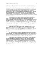
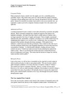
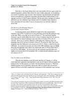
This point can also be made graphically. Consider Figure 8.22, in which lines
A
1
H
1
and A
1
H
3
of Figure 8.21 are replicated. A person who buys combination b,
including a relatively small house in Six Mile, would require an additional income of
something less than the horizontal distance ab (which is the additional income that the
person needs to duplicate in La Jolla his or her Six Mile house). A person who buys
combination d, which includes a much larger house in Six Mile, would require an
additional income of something less than cd. In the graph, cd is about twice the size of
ab.
____________________________________
FIGURE 8.22 Choosing Employees Based on the
Sizes of their Houses
An employee who chooses combination b in Six
Mile, with H
4
housing would require additional pay
equal to ab. An employee who chooses
combination d in Six Mile would require much more
in additional pay, cd.
__________________________________________