Tài liệu Microeconomics for MBAs 32 pptx

Chapter 9 Production Costs and
Business Decisions

7



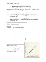
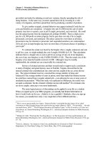
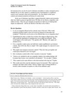
TABLE 9.1 Marginal Costs of Producing Tomatoes


Contribution Number of
of Each Workers Marginal
Number Worker to Required to Cost of
of Total Production Produce Each Each Bushel,
Workers Number of (Marginal Additional Figured at
Employed Bushels Product) Bushel $5 per Worker
(1) (2) (3) (4) (5)

1 0.25 0.25
2 1.00 0.75 (1st bushel) 2 $10
3 2.00 1.00 (2
nd
bushel) 1 $ 5

Point at Which Diminishing Maginal Returns Emerge

4 2.60 0.60
5 3.00 0.40 (3rd bushel) 2 $10
6 3.30 0.30
7 3.55 0.25
8 3.75 0.20 (4th bushel) 5 $25

9 3.90 0.15
10 4.00 0.10

_______________________________________
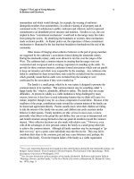
FIGURE 9.2 The Law of Diminishing Marginal
Returns
As production expands with the addition of new
workers, efficiencies of specialization initially cause
marginal cost to fall. At some point, however—here,
just beyond two bushels—marginal cost will begin to
rise again. At that point, marginal returns will begin
to diminish and marginal costs will begin to rise.
_______________________________________


The Cost-Benefit Tradeoff
Just as a producer’s marginal cost schedule shows the increasing cost of supplying more
goods, the demand curve, as explained earlier, shows the decreasing value or marginal
benefit of those goods to the people consuming them. Together, marginal costs and
benefits determine how many units will be produced and consumed up to the intersection
of the marginal cost and demand (marginal benefit) curves, the marginal benefit of each
Chapter 9 Production Costs and
Business Decisions

8
additional unit exceeds it marginal cost. In other words, people can gain through
production and consumption of those units. The intersection of the two curves represents
the limit of production, or the point at which welfare is maximized. To see this point,
consider the costs and benefits of an activity like fishing.

The Costs and Benefits of Fishing
Gary Schmidt likes to fish. What he does with the fish he catches is of no consequence to
us; he can make them into trophies, give them away, or store them in the freezer. Even if
Gary places no money value on the fish, we can use dollars to illustrate the marginal
costs and benefits of fishing to Gary. (Money figures are not values, but a means of
indicating relative value.)
What is important is that Gary wants to fish. How many fish will he catch? From
our earlier analysis of Jan’s desire to paint (page 181), we know that the cost of catching
each additional fish will be higher than the cost of the one before. Gary will confront an
upward-sloping marginal cost curve like the one in Figure 9.3. Gary’s demand curve for
fishing will slope downward, for as the cost of catching each additional fish rises, Gary
will be less and less inclined to spend more time on the activity (see Figure 9.3).

_______________________________________
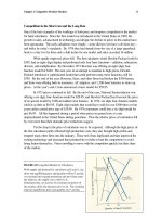
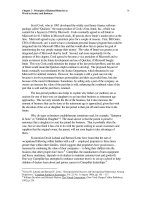
FIGURE 9.3 Costs and Benefits of Fishing
For each fish up to the fifth, Gary receives more
in benefits than he pays in costs. The first fish
gives him $4.67 in benefits (point a) and costs
him only $1 (point b). The fifth yields equal
costs and benefits (point c), but the sixth costs
more than it is worth. Therefore Gary will catch
no more than five fish.




From the positions of the two curves, we can see that Gary will catch up to five
fish before he packs up his rod and heads for home. He places a relatively high value of
$4.67 on the first fish (point a in the figure) and places the relatively low marginal cost of

$1 on forgone opportunities for it (point b). In other words, he gets $3.67 more value
from using his time, energy, and other resources to fish than he wold receive from his
nexr best alternative. The marginal benefit of the second fish also exceeds its marginal
cost, although by a small amount ($2.75-$4.25 $1.50). Gary continues to gain with the
third and fourth fishes, but the fifth fish is a matter of indifference to him. Its marginal
value equals its marginal cost (point c). Although we cannot say that Gary will actually
bother to catch a fifth fish, we do know that five is the limit toward which he will aim.
Chapter 9 Production Costs and
Business Decisions

9
He will not catch a sixth—at least during the period of time offered by the graph—
because it would cost him more than he would receive in benefits.

The Costs and Benefits of Preventing Accidents
All of us would prefer to avoid accidents. In that sense we have a demand for accident
prevention, whose curve should slope downward like all other demand curves.
Preventing accidents also entails costs, however, whether in time, forgone opportunities,
or money. Should we attempt to prevent all accidents? Not if the cost of ensuring that
you will never stumble down the stairs is $100 (again, we are using dollars to indicate
relative value). If the only injury you expect to suffer were a bruised knee, would you
spend $100 to prevent the accident?
As with the question of how long to fish, marginal cost and benefit curves can
help illustrate the point at which preventing accidents ceases to be cost effective.
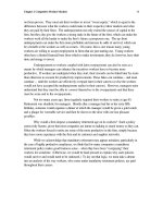
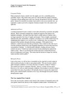
Suppose Al Rosa’s experience indicates that he can expect to have ten accidents over the
course of the year. If he tries to prevent all of them, the value of preventing he last one,
as indicated by the demand curve in Figure 9.4, will be only $1 (point a). The marginal
cost of preventing it will be much greater: approximately $6 (point b). If Al is rational,
he will not try to prevent the last accident. As a matter of fact, he will try to prevent only
five accidents (point c). As with the tenth accident, it will cost more than it is worth to Al

to prevent the sixth through ninth accidents. He would try to prevent all ten accidents
only if his demand for accident prevention were so great that his demand curve
intersected the marginal cost curve at point b.
Some accidents may be unavoidable. In that case, the marginal cost curve will
eventually become vertical. Other accidents may be avoidable in the sense that it is
physically possible to take measures to prevent them—although the rational course may
be to allow them to happen.
_________________________________
FIGURE 9.4 Accident Prevention
Given the increasing marginal cost of preventing
accidents and the decreasing marginal value of
preventing the accidents, c accidents will be
prevented.
_________________________________




The Production Function in Pictures
Business firms combine various factors of production in order to produce various goods
and services. Although there are thousands of different factors of production, or inputs,
Chapter 9 Production Costs and
Business Decisions

10
for simplicity we often use a model with only two factors, labor and capital. We can then
study how the two inputs can be combined to produce an output. The relationship
between inputs and output is called the production function. The general equation for
the production function is:
Q = f (L, K)

where Q is output, L is labor, K is capital, and f is the functional relationship between
inputs and output. In the short run, we assume that capital cannot be varied; labor is
therefore, the only variable factor. To increase output, then, a firm must increase the
amount of labor.
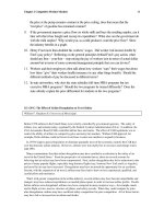
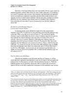
The relationship between the amount of the variable input (labor) and output can
be illustrated with a total product curve such as that in the upper half of Figure 9.5.
Suppose that the curve is that of a commercial fishing firm. The firm’s capital—the boat
and equipment—is fixed in the short run. Only the number of workers can vary. As the
amount of labor increases from zero, the fish catch (output) increases. Between zero and
5 workers, output increases at an increasing rate. As more workers are hired total output
continues to increase, although at a decreasing rate, until 15 workers are hired. Beyond
that point, hiring more workers reduces output.
The reason the total product curve has that particular shape can be seen more
clearly in the lower half of Figure 9.5, which shows the average and marginal product
curves. The average product of labor is total output divided by the amount of labor, or
Q/L. The marginal product of labor is the change in total output brought about by
changing the amount of labor by one unit. Because at least some workers are needed to
operate the boat and the equipment, the first few workers hired greatly increase total
output; marginal product is rising. Between 5 and 15 workers, the marginal product of
labor falls, although the average product continues to rise (because it is less than marginal
product). Total product continues to rise, but no longer at an increasing rate. The law of
diminishing marginal returns has taken effect. At seven workers, marginal product
equals average product and average product is maximized. As more workers are hired
average product falls. Note that as long as marginal product is positive, more labor
means more output and the total product curve will have a positive slope. Beyond 15
workers, marginal product becomes negative and total product falls. The boat may be so
crowded that workers bump into each other and reduce the amount of work that each
does. To catch more fish once this stage has been reached, the firm must buy a larger
boat.
Some economists divide the production function of Figure 9.5 into three stages.

In stage one, from zero to seven workers, total product and average product of labor both
rise. In stage two, between seven and 15 workers, total product rises while average
product falls. In stage three, beyond 15 workers, total product and average product both
fall (and marginal product is negative).
Chapter 9 Production Costs and
Business Decisions

11

Price and Marginal Cost: Producing to Maximize Profits
“Production” is not generally an end in itself in business. Most firms seek to make a
profit. How can we think about how they go about the task of trying to maximize profits?
The total and marginal product curves need to be converted to cost curves. Only then can
we engage in familiar cost-benefit analyses.
Granted, many business people derive intrinsic reward from their work. They may
value the satisfaction of producing a product that meets a human need just as much as the
profits they earn. Some business people may even accept lower profits so their products
can sell at lower prices and serve more people. For most business people, however, the
profit generated by sales is the major motivation for doing business.

________________________________
FIGURE 9.5 Total, Average, and Marginal
Product Curves
The total product curve shows how output
changes when the amount of the variable
input, labor, changes. Total product rises first
at an increasing rate (0 to 5 workers), then at
a decreasing rate (5 to 15 workers), before
declining (beyond 15 workers). The marginal
and average product curves reflect what is

happening to total product. Marginal product
rises when total product is rising at an
increasing rate and falls when total product is
rising at a decreasing rate. Marginal product
is positive when total product is rising and
negative when total product is falling.








How much will a profit-maximizing firm produce? Assume its marginal cost
curve is like the one in Figure 9.6(a). Assume further that the owners can sell as many
units as they want at a price of P
1
. Because this firm is in business to make a profit, the
price of its product can be thought of as the marginal benefit of each additional unit. P
1
is
also the firm’s marginal revenue. Marginal revenue is the additional revenue a firm
Chapter 9 Production Costs and
Business Decisions

12
acquires by selling an additional unit of output. Each time the firm sells one additional
unit, its revenues rise by P
1

.
Clearly, a profit-maximizing firm will produce and sell any unit for which the
marginal revenue acquired (MR) exceeds the marginal cost (MC). (Profits are the
difference between total costs and total revenues. Therefore a firm’s profits rise whenever
an increase in revenues exceeds the increase in its costs.) At a price of P
1
,

then, this firm
will produce up to, and no more than, Q
1
, products. For every unit up to Q
1
, price is
greater than marginal cost.

________________________________
FIGURE 9.6 Marginal Costs and
Maximization of Profit
At price P1 (part (a)), this firm’s marginal
revenue, shown by the shaded area under P1,
exceeds its marginal cost up to an output level
of Q1. At that point total profit, shown in part
(b), peaks (point a). At price P2, marginal
revenue exceeds marginal cost up to an output
level of Q2. The increase in price shifts the
profit curve in part b upward, from TP1 to TP2,
and profits peak at b.
________________________________

Chapter 9 Production Costs and
Business Decisions

13
The vertical distance between P1 and the marginal cost of each unit, as shown by
the marginal cost curve, is the additional profit obtained from each additional unit
produced. By summing the vertical distance between P1 and the marginal cost curve for
all units up to Q
1
, we can obtain the firm’s total profits. (See the color-shaded area in
Figure 9.5(a).) Total profits can also be represented as a curve, as in the line TP
1
in
Figure 9.5(b). Notice that the curve peaks at Q
1
the point at which the firm chooses to

stop producing. Beyond Q
1
, marginal cost is greater than marginal revenue, and total
profits fall, as shown by the downward slope of the total profits curve.

What will the firm do if the price of its product rises from P
1
to P
2
? For the firm
that can sell all it wants at a constant price, a rise in price means a rise in marginal
revenue. Once the price rises to P
2
, the marginal revenue of an additional Q
2
– Q
1

products exceeds their marginal cost. At the higher price, a larger number of units can be
profitably produced and sold. The firm will seek to produce up to the point at which
marginal cost equals the new, higher marginal revenue, P
2
, or output, Q
2
, in Figure 9.5
(a). As before, profit is equal to the vertical distance between the rice line, P
2
, and the
marginal cost curve, or the color-shaded area plus the gray-shaded area in Figure 9.5 (a).
The total profit curve shifts to the position of the line TP

2
in Figure 9.5(b).

From Individual Supply to Market Supply
If a portion of the upward-sloping marginal cost curve is the firm’s supply curve, and if
market supply is the amount all producers are willing to produce at various prices, we can
obtain the market supply curve by adding together the elevation portions of the individual
firms’ marginal cost curves. (This procedure resembles the one followed in determining
the market demand curve in an earlier chapter.)
Figure 9.7 shows the supply curves S
A
and S
B
, derived from the marginal cost
curves of two producers, A and B. At a price of P
1
, only producer B is willing to produce
anything, and it is willing to offer only Q
1
. The total quantity supplied to the market at P
1

is therefore Q
1
. At the higher prices of P
2
, however, both producers are willing to
compete. Producer A offers Q
1
, while producer B offers more, Q

2
. The total quantity
supplied is therefore Q
3
the sum of Q
1
and Q
2
.
The market supply curve, S
A+B
is obtained by adding the amounts A and B are
willing to sell at each price and splitting the totals. Note that the market supply curve lies
farther from the origin and is flatter than the individual producers’ supply curves. The
entry of more producers will shift the market supply curve farther outward and lower its
slope even more. (More will be said about cost and supply in later chapters.)

MANAGER’S CORNER: Cutting Health Insurance Costs
The cost of doing business is a constant worry for all firms. At times, those business
costs feed major policy debates in the nation’s capital. As is so often the case, the
infamous “healthcare crisis” in the United States amounts to nothing more than costs for
Chapter 9 Production Costs and
Business Decisions

14
a particular service – healthcare responding to the market forces of supply and demand.
Unfortunately, the forces have been distorted by legal and political factors that have
gotten the incentives wrong. In our view, the “crisis” is more a matter of political
rhetoric than economics. Political grandstanding alone will hardly solve whatever
healthcare problem exists. Careful reflection by policy makers and managers on the

exact sources of the problem might. The current distortion presents a possibility for
managers to benefit both their firms and its workers by policies that get the incentives
right.

____________________________________
FIGURE 9.7 Market Supply Curve
The market supply curve (SA+B) is obtained
by adding together the amount producers A
and B are willing to offer each at each and
every price, as shown by the individual
supply curves SA and SB. (The individual
supply curves are obtained from the upward
sloping portions of the firms’ marginal cost
curve.)
______________________________





If private firms and Washington-based politicians want to reform the system and
temper cost increases, they can do so by working with the forces of supply and demand,
which means, fundamentally, changing people’s incentives to provide and consume
healthcare services.
Granted, healthcare costs, and the insurance premiums that finance a major share
of healthcare expenditures, have risen faster than the prices of other goods over the last
couple of decades.
1
Indeed, the cost of health insurance provided by firms was escalating
at double-digit rates in the late 1980s and the very early 1990s when increases in the

consumer price index, a broad measure of the cost of living, were falling.
2
In the mid-
1990s, healthcare cost increases slowed, but they were, at this writing, still increasing at a
rate that was over 50 percent higher than the rate of increase in the general cost of living.

1
See Paul J. Feldstein. Health Policy Issues: An Economic Perspective on Health Reform (Arlington, Va. :
AUPHA Press; Ann Arbor, Mich.: Health Administration Press, 1994); and Paul J. Feldstein, The Politics
of Health Legislation: An Economic Perspective, 2nd ed. (Chicago, Ill.: Health Administration Press,
1996).
2
Put another way, the consumer price index was increasing at decreasing rates, which means that the rate
of inflation was gradually but irregularly decreasing for most of the 1980s and 1990s.
Chapter 9 Production Costs and
Business Decisions

15
In order to understand the problem of insurance cost increases, we need first to
consider the market forces that have been at work driving up healthcare costs. What are
those forces? Consider the following list of factors affecting the supply and demand of
healthcare:
1. Doctors have been subject to a growing degree of litigation. They have been sued
with growing frequency partly because they have made mistakes, but also because
they are now being held responsible for problems over which they may have no
control. Patients have found that they can make money by blaming doctors for
almost any problem that emerges when they are being treated. Fearful that they
will be sued for delivering incomplete or misguided care, doctors have been
covering their financial and professional backsides by ordering tests that may be
only marginally valuable from a medical perspective but can help them defend

themselves in the event they are sued when problems emerge. They have also
been trying to acquire legal protection and to spread the risk of lawsuits by
increasing referrals to specialists.
2. Federal expenditures on Medicare for older patients and Medicaid for low-income
patients have increased the demand for healthcare services since the late 1960s,
which has tended to boost prices and forced many younger and lower-income
patients out of the health insurance market.
3. Medical care has become technologically more sophisticated, and doctors have
applied the new technology for offensive reasons (to keep patients alive longer)
and for defensive reasons (they don’t want to be accused of negligence for failing
to employ the latest life-saving technology). The extensive use of the latest and
best technology may have saved and prolonged lives, but medical care costs have
been driven up in the process.
4. The healthcare industry has always been plagued by the problem of “asymmetric
information,” or the doctors knowing more about many patients’ medical
conditions and what will remedy their problems than do the patients themselves.
As a consequence, doctors have always been in a position to induce patients to
buy more medical care than the patients might really buy, if they had the
information and knowledge at the disposal of the doctors.
5. Medical technology has drastically lowered the cost of many medical procedures
and has, as a consequence, lowered the cost of extending the lives of patients by
some varying and uncertain number of months and years. For example, less than
four decades ago, heart and kidney transplants and heart bypass operations were
impossible. No one knew how to do them. Then, the costs of those procedures
were infinite. Their prices may now remain high in absolute dollar terms, running
into the tens, if not hundreds, of thousands of dollars. However, those high prices
also represent lower prices. And the lower prices for those procedures have, no
doubt, increased the number of patients who have been willing and able to pay for
the procedures (as well as insurers who have helped with the payments).
Although the issue has not been statistically evaluated to date, the lower prices for

many medical procedures have probably increased total medical expenditures in
Chapter 9 Production Costs and
Business Decisions

16
absolute dollar terms and as a percentage of national income. Hence, some of the
so-called healthcare “crisis” probably mirrors, to a degree, the success of the
healthcare industry in lowering the cost of prolonging life.
6. The cost of employer-provided medical insurance is tax deductible, which means
that its price has been artificially lowered, causing more consumers to buy more
complete insurance coverage and to demand more medical services (than they
otherwise would). The greater demand has enabled medical professionals to
boost their prices. As tax rates rose in the 1960s and 1970s, workers naturally had
growing incentive to take more of their income in tax-deductible fringe benefits
and less of an incentive to take their income in taxable money wages. The higher
tax rates spurred demand for health insurance and healthcare – and added to
pressure on healthcare costs.
7. Employers have typically bought insurance policies with very low deductibles, for
example, $200 a year. This means that after the first $200 of medical care
expenditures in any one year, the cost of additional medical services to the insured
patient is often close to zero. This feature of insurance policies has encouraged
excessive use of healthcare services, which, in turn, has driven up employees’
insurance premiums and caused some workers to forgo health insurance
altogether.
3

8. The growth in social problems crimes involving bodily injury, the use of street
drugs, and teenage pregnancy has also contributed to the demand for medical
services, which has driven up their prices as well as the price of insurance. The
unwillingness or inability of medical professionals to deny services to people who

cannot pay for the services has also increased the number of people seeking
services. Social attitudes favoring universal medical care coverage have reduced
the cost of irresponsible behavior, increasing the demand on the healthcare
industry and inflating costs.
Without question, if the grocery industry were operated the way the healthcare
industry operates, then we would likely have a “crisis” in the grocery business. The
reason is simple: People would pay a fixed sum each month (their grocery premium)
through their employer that would entitle them to virtually unlimited access to the
grocery store shelves (after they have covered the $200 annual deductible) at zero, or
very low, cost. Under such an arrangement, we should not be surprised if people
consumed significantly more and better food, some of which would have limited value.
We should also not be surprised if the shoppers’ grocery premiums went through the roof
as everyone allowed their tastes to run wild, with many low-income shoppers forced out
of the grocery policies by the inflated premiums.

3
As you may recall from our study of consumer behavior in the last chapter, a working rule of consumer
maximizing behavior is that the consumer will continue to buy units of any good or service until the point
at which the marginal cost of the last unit consumed just equals the marginal value of the last unit. If the
person consumes more than that amount, the additional cost of any additional units will exceed their
additional value. By “excessive” consumption, we mean that patients are induced to go beyond the point
where the marginal value is, while still positive, less than the marginal cost. The reason for this excessive
consumption is that the individual consumer isn’t paying the entire cost of additional medical care.