Tài liệu Microeconomics for MBAs 35 docx

Chapter 10 Production Costs in the
Short Run and Long Run




13
the agency cost?” Given that agency costs will always occur with expanding firms, how
can the combination of debt and equity be varied to minimize the amount of costs from
shirking and opportunism? That question is really one dimension of a more fundamental
one, “How can the financial structure affect the firm’s costs and competitiveness?”
In this short chapter, the eye of our focus is on debt, but that is only a matter of
convenience of exposition, given that any discussion of debt must be juxtaposed with
some discussion of equity as a matter of comparison, if nothing else. We could just as
easily draw initial attention to equity as a means of financing growth. In fact, debt and
equity are simply two alternative categories of finance (subject to much greater variation
in form than we are able to consider here) available to owners. Owners need to search for
an “optimum combination,” given the features of both.

Debt and Equity as Alternative
Investment Vehicles
By debt, of course, we mean funds, or the principal, that must be repaid fully at some
agreed-upon point in the future and on which regular interest payments must be made in
the interim. The interest rate is simply the annual interest payment divided by the
principal. Also, we must note that in the event the firm gets into financial problems, the
lenders have first claim on the firm’s remaining assets.
By equity, or stock, we mean funds drawn from people who have ultimate control
over the disposition of firm resources and who accept the status of residual claimants,
which means a return on investment (which is subject to variation) will be paid only after
all other claims on the firm have been satisfied. That is to say, the owners (stockholders)
will not receive dividends until after all required interest payments have been met; the

owners are guaranteed nothing in the form of repayment of their initial investments.
Obviously, owners (stockholders) accept more risk on their investment than do lenders
(or bondholders).
2

Having outlined our intentions for this chapter, does it matter whether a firm
finances its investments by debt or equity?
3
You bet it does (otherwise we must wonder
why the two broad categories of finance would ever exist). The most important feature of
debt is that the payments, both the payoff sum and the interest payments, are fixed. This
is important for two reasons. One reason is the obvious one it enables firms to attract
funds from people who want security and certainty in their investments. The modern
aphorism, “different strokes for different folks,” if followed in the structuring of financial

2
We recognize that debt and equity come in a variety of forms. Common and preferred stock are the two
major divisions of equity. Debt can take a form that has the “look and feel” of equity. For example, the
much-maligned “junk bonds” often carry with them rights of control over firm decisions and may also be
about as risky as common stock. In order to contain the length of this chapter, we consider only the two
broad categories, and we will encourage readers to consult finance texts for more details on financial
instruments. However, readers should recognize that variations in the type of debt and equity could help
overcome some of the problems with each that are discussed in this chapter.
3
For a more complete discussion of answers to this question, see Michael C. Jensen and William H.
Meckling, “Theory of the Firm: Managerial Behavior, Agency Costs and Ownership Structure,” Journal of
Financial Economics, vol. 3 (October 1976), pp. 305-360.
Chapter 10 Production Costs in the
Short Run and Long Run

14
instruments, can mean lower costs of investment funds, growth, and competitiveness.
Debt attracts funds from people who get their “strokes” from added security.
Fixed payments on debt are more important for our purposes for another reason:
If the firm earns more than the required interest payments on any given investment
project, the residual goes to the equity owners. If the company fails because of
investments gone sour, then the firm is limited in its liability to lenders to the amount of
their loans. If the firm is forced to liquidate its assets and the sale is insufficient to cover
the debt, then it’s simply going to be a sad day for the lenders (as well as stockholders,
who will get nothing). The lenders can claim only what is left from the sale. That’s it.
Any profit remaining after all expenses have been covered doesn’t have to be shared with
the lenders. The remaining profits go to the equity stakeholders.
Clearly, the nature of debt biases, to a degree (depending on the exact features),
the decision making of the owners, or their agent-managers, toward seeking risky
investments, ones that will likely carry high rates of return. These high rates will, no
doubt, incorporate a premium for risk taking, but they can also provide equity owners
with an opportunity for a premium residual, given that they get what is left after the
interest payments are deducted from high returns. If a firm borrows funds at a 10 percent
interest rate, for example, and invests those funds in projects that have an expected rate of
return of 12 percent, the residual left for the equity owners will be the difference, 2
percent. If, on the other hand, the funds are invested in a much riskier project that has a
rate of return of 18 percent, then the residual that can be claimed by the equity owners is
8 percent, four times as great as the first case.
Granted, the project with the higher rate has a risk premium built into it (or else
everyone investing in the 12 percent projects would direct their funds to the 18 percent
projects, causing the rate of returns in the latter to fall and in the former to rise).
However, notice that much of that additional risk is imposed on the lenders. They are the

ones who must fear that the incurred risk will translate into failed investments (which is
what risk implies). But they are not the ones who are compensated for the assumed risk
they bear. Indeed, once a lender has made a loan, the managers can extend their
indebtedness with more venturesome investments, increasing the risk imposed on the
original lenders.
As a general rule, the greater the indebtedness, the greater incentive managers
have to engage in risky investments. Again, this is because much of the risk is imposed
on the lenders and the benefits, if they materialize, are garnered by the equity owners.
It should surprise no one that as a firm takes on more debt, lenders will become
progressively more concerned that they will lose some or all of their investments. As a
consequence, lenders will demand compensation in the form of higher interest payments,
which reflect a risk premium. Those lenders who fear that the firm will continue to
expand its indebtedness after they make the initial loans will also seek compensation
prior to the rise in indebtedness by way of a higher interest rate. To keep interest costs
under control, firm managers will want to find ways of making commitments as to how
much indebtedness the firm will incur, and they must make the commitments believable,
or else higher interest rates will be in the making. Again, we return to a reoccurring
Chapter 10 Production Costs in the
Short Run and Long Run




15
theme in this book: managers’ reputations for credibility have an economic value. In this
case, the value emerges in lower interest payments.
Lenders, of course, will seek to protect themselves from risky managerial
decisions in other ways. They may seek, as they often do, to obtain rights to monitor and
even constrain the indebtedness of the firms to whom they make loans. Managers also
have an interest in making such concessions because, although their freedom of action is

restricted in one sense, they can be compensated for the accepted restrictions in the form
of interest rates that are lower than otherwise. Firm managers are granted greater
freedom of action in another respect; they are given a greater residual with which they
can work (to add to their salary and perks, if they have the discretion to do so; extend the
investments of the firm; or increase the dividends for stockholders).
Lenders may also specify the collateral the firm must commit. Lenders will not
be interested in just any form of collateral. They will be most interested in having the
firm pledge “general capital,” or assets that are resaleable, which means that the lenders
can potentially recover their invested funds. Lenders will not be interested in having
“specific capital,” or assets that are designed only for their given use inside a given firm.
Such assets have little, if any, resale market.
Of course, firm assets are often more or less “general” or “specific,” which means
they can be better or worse forms of collateral. A firm can pledge assets with “specific
capital” attributes. However, managers must understand that the more specific the asset
(the narrower the resale market), the greater the risk premium that will be tacked onto the
firm’s interest rate, and the lower the potential residual for the equity owners.
Lenders will also have a preference for lending to those firms that have a stable
future income stream and that can be easily monitored. The more stable the future
income, the lower the risk of nonpayments of interest. The more easily the firm can be
monitored, the less likely managers will be able to stick creditors with uncompensated
risks. The more willing lenders are to lend to firms, the greater the likely indebtedness.
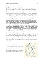
Electric utility companies have been good candidates for heavy indebtedness,
because their markets are protected from entry by government controls and regulations,
what they do is relatively easily measured, and their future income stream can be
assumed to be relatively stable. Accordingly, their interest rates should be relatively low,
which should encourage managers to take on additional debt just so that equity owners
can claim the residual for themselves. (At this writing, the deregulation of electric
power production is underway in a few states, which allows open entry into the
generation of electricity. We should expect deregulation to lead to a higher risk premium
in interest rates, although the price of electricity can be expected to fall for consumers

with increased competition for power sales.)

Incentives in the S&L Industry
The incentives of indebtedness are dramatically illustrated in the biggest financial
debacle of modern times, the dramatic rise in savings and loan bank failures of the 1980s.
The S&L industry was established in the 1930s to ensure that the savings of individuals,
Chapter 10 Production Costs in the
Short Run and Long Run




16
who effectively loaned their funds to the S&Ls, could be channeled to the housing
industry (a concentrated focus of S&L investment portfolios that in itself added an
element of risk, especially since housing starts vary radically with the business cycle).
S&Ls were in a position to loan money for housing that was up to 97 percent from their
depositors and only three percent from the owners (given reserve and equity
requirements). Such a division, of course, made the S&L owners eager to go after high-
risk but high-return projects. They could claim the residual from what was then a fixed
interest payment on deposits.
When interests rates began to rise radically with the rising inflation rates of the
late 1970s, alternative market-based forms of saving became available – not the least of
which were money-market and mutual funds, which were unrestricted in the rates of
return they could offer savers. As a consequence, savings started flowing out of S&Ls,
which greatly increased the pressure on S&Ls to hike, when they were freed to do so, the
interest rates on their deposits and to offset the higher interest rates by searching out
investments that were risky but carried high rates of returns.
The S&Ls’ incentive for risky investment was heightened by the fact that
depositors’ incentives to monitor the loans were severely muted by federal deposit

insurance, which effectively assured the overwhelming majority of all depositors that
they would lose nothing if all their S&L loans went sour.
To compensate for these perverse incentives, the federal government closely
monitored and regulated the investments of the S&Ls through 1982. But that year, S&Ls
were given greater freedom to pursue high-risk investments at the same time the
protection to depositors was increased. The result was that which should have been
predicted from the simple thought that if you give enough people a large enough
temptation, many will succumb. S&Ls went after the high-risk/high-return and high
residual investments. The S&Ls that made the risky investments were in a position to
pay high interest rates, drawing funds from other more conservative S&Ls. In order to
protect their deposit base, conservative S&Ls had to raise their interest rates, which
meant that they, too, had to seek riskier investment, all of which led to a shock wave of
risky investment spreading through the S&L/development industry.
Unfortunately, many of those investments did what should have been expected by
their risky nature: they failed. The government had to absorb the losses and then return
to doing that which it had done before 1982 closely monitor the industry and more
severely restrict the riskiness of the investments (given that it was unwilling to give
depositors greater incentives to monitor their S&Ls).
Clearly, fraud was a part of the S&L debacle. Crooks were attracted to the
industry.
4
However, the debacle is a grand illustration of how debt can, and did, affect
management decisions. It also enables us to draw out a financial/management principle:
If owners want to control the riskiness of their firms’ investments, they had better look to
how much debt their firms accumulate. Debt can encourage risk taking, which can be

4
See William K. Black, Kitty Calavita, and Henry N. Pontell, “The Savings and Loan Debacle of the 1980s:
White-Collar Crime or Risky Business?” Law & Policy, vol. 17, no. 1 (Jan. 1995).
Chapter 10 Production Costs in the

Short Run and Long Run




17
“good” or “bad,” depending on whether the costs are considered and evaluated against
the expected return.
Why then would the original equity owners ever be in favor of issuing more
shares of stock and bringing in more equity owners with whom the original owners would
have to share the residual? Sometimes, of course, the original owners are unable to
provide the additional funds in order for the firm to pursue what are known (in an
expectation sense) to be profitable investment projects. The original owners can figure
that while their share of firm profits will go down, the absolute level of the residual they
claim will go up. A 60 percent share of $100,000 in profits beats 100 percent of $50,000
in profits any day.
Another less obvious reason is that the additional equity investment can reduce
the risk that the lenders face with loans to the firm. This means that the equity owners
can claim a greater residual due to the fact that firm interest payments can fall with the
reduction in the risk premium.
Often investment projects require a combination of specific and general capital to
be used together. Consider, for example, the predicament of a remodeling firm that uses
specially designed pieces of floor equipment (which may have little or no market value
outside of the firm) as well as trucks that can easily be sold in well-established used truck
markets. The investment projects can be divided according to the interests of the two
types of investors. The equity owners can be called upon to take the risk associated with
the floor equipment while the lenders are called upon to provide the funds for the trucks.
Indeed, the lender might not even make the loan for the general part of the investment
without equity owners taking the specific part precisely because the general investment
would have limited value (or would carry undue risk) without the specific capital

investment. (There may be no reason for the trucks if the firm has no floor equipment to
work with.)
The original owners can also have an interest in selling a portion of their
ownership share because, by doing so, they can reduce the overall risk of their full
portfolio of investments by reinvesting the proceeds elsewhere, indeed, spreading their
investments among a number of firms. If the original owners held their full investments
in the firm, and refused to sell off a portion, then they might be “too cautious” in the
choice of investments they would want the firm to pursue too reluctant to take the risky
investments that can be the more rewarding endeavors.
By selling a portion of their interest in the firm, the original owners can actually
change the direction of the firm’s investment projects, and its growth, and can make the
firm more profitable which translates into greater wealth for the original owners. The
original owners can do this by lowering their (risk) costs by way of spreading their
investments, and then by taking on more risky but more profitable investments in the
original firm. Again, the financial structure of the firm is important and it can matter to
management policies and to the bottom line.
Finance Professor Michael Jensen argues there is another reason for indebtedness
for some firms: The interest payments on the debt can tie the hands or reduce the
discretionary authority of managers who might otherwise engage in opportunism with
Chapter 10 Production Costs in the
Short Run and Long Run




18
their firms’ residual.
5
If a firm has little debt, then the managers can have a great deal of
funds, or residual, to do with as they please. They can use the residual to provide

themselves with higher salaries and more perks. They can also use the funds to
contribute to local charities that may have little impact on their firm’s business (they may
have a warm heart for the cause they support or they may only want to take credit for
being charitable with their firms’ funds). They may also use the funds to expand (without
the usual degree of scrutiny) the scope and scale of their firms, thereby giving reason for
higher salaries and more perks (since size and executive compensation tend to go
together) for themselves.
The investment projects the managers choose may indeed be profitable. The
problem is that if the funds were distributed to the stockholders, the stockholders could
find even more profitable investments (and even more worthy charitable causes).
As industries mature (or reach the limits of profitable expansion), the risk of
managers “misusing” firm funds can grow. There may be few opportunities for managers
to reinvest the earnings in their own industry. They may then be tempted to use the
“excess residual” to fulfill some of their own personal flights of managerial fancy (give to
charitable causes or pad their pockets), or reinvest the funds in other industries which
may, or may not, have a solid connection to the original firm’s core activities. Because
of the additional costs of centralization and coordination of the investments across
industries, the stock prices of mature companies can become depressed.
How can the firm be disgorged of the residual? Jensen suggests through
indebtedness: the greater the indebtedness, the smaller the residual, and the less waste
that can go up in the smoke of managerial opportunism. Jensen argues that one of the
reasons for firm takeovers by way of “leveraged buyouts,” which means heavy
indebtedness, is that the firm is then forced to give up the residual through higher interest
payments. Again, the hands of the agent-managers are tied; their ability to misuse firm
funds is curbed. The value of the firm is enhanced by the indebtedness, mainly because it
reduces the discretion of managers who have been misusing the funds. And managers
can misuse their discretion in counterproductive ways, not the least of which is by
diversifying the array of products and services provided on the grounds that diversity can
smooth out the company’s cash flows over the various cycles that go with the products
and services. As Al Dunlap recognizes, “The flaw in that thinking is that shareholders

are quite able to diversify on their own, thank you. Management doesn’t have to do that
for them.”
6
But management does have to pass back the cash flow to the shareholders or,
as the case may be, lenders.


5
Michael C. Jensen, “Eclipse of the Public Corporation,” Harvard Business Review (September-October
1989), pp. 64-65.
6
Al Dunlap and Bob Andelman, Mean Business: How I Save Bad Companies and Make Good Companies
Great (New York: Times Books, 1996), p. 81.

Chapter 10 Production Costs in the
Short Run and Long Run




19
Firm Maturity and Indebtedness
This all leads us to an interesting proposition. We should expect firm
indebtedness to increase with the maturity of its industry. Firms in a mature industry
have more stable future income streams. They can be more easily monitored, given
people’s experience in working with the firms and knowing how such firms operate and
are inclined to misappropriate funds when they do. Also, by taking on more debt, firms
in mature industries can alert the market to their intentions to rid themselves of their
residual, and not misuse managerial discretion, all of which can drive up the price of the
firm’s stock to a point that could not otherwise be reached.

Of course, if firms in mature industries don’t take on relatively more debt and
managers continue to misuse the funds by reinvesting the residual in the mature industry
or other industries, then the firm can be ripe for a takeover. Some outside “raider” will
see an opportunity to buy the stock, which should be selling at a depressed price, paying
for the stock with debt. The increase in indebtedness can, by itself, raise the price of the
stock, making the takeover a profitable venture. However, if the takeover target is,
because of past management indiscretions in investment, a disparate collection of
production units that do not fit well together, the profit potential for the raiders is even
greater. The firm should be worth more in pieces than as a single firm. The raiders can
buy the stock at a depressed price, take charge, and break the company apart, selling off
the parts for more than the purchase price. In the process, the market value of the “core
business” should be enhanced.
* * * * *
The moral of this “Manager’s Corner” should now be self-evident: The financial
structure of firms matters, and it matters a great deal. The structure can affect managerial
actions and determine policies. The structure can also determine whether the firm will be
the subject of a takeover. The one great antidote for a takeover should be obvious to
managers, but it is not always (as evident by the fact that takeovers are not uncommon):
Firms should be structured, both in terms of their financial and internal policies, in such a
way that the stock price is maximized. In that case, potential raiders will have nothing to
gain by taking the firm over. The jobs of the executives and their boards will be secure.
Of course, one of the primary functions of a board of directors is to monitor the
executives and the policies that are implemented with an eye toward maximizing
stockholder value. As we will see, those executives and their board that do not maximize
the price of their stocks do have something to fear from corporate raiders. They have
definite reason, as we will see, to denigrate the social value of corporate raiders and to
foil the takeover efforts of the raiders.

Concluding Comments
Short- and long-run costs are important topics in the study of economics. In order to

understand how competitive and monopolistic markets operate, we must first understand
the firm’s cost structure. In following chapters, we will combine the average and
marginal cost curves described here with the demand curves described in earlier chapters.
Within that theoretical framework, we will be able to compare the relative efficiency of
Chapter 10 Production Costs in the
Short Run and Long Run




20
competitive and monopolistic markets, and the role of profits in directing the production
decisions of private firms.


Review Questions
1. Complete the cost schedule shown below and develop a graph that shows marginal,
average fixed, average variable, and average total cost curves.


Output
Level
Total
Fixed
Costs
Total
Variable
Costs

Total

Cost

Marginal
Cost
Average
Fixed
Cost
Average
Variable
Cost
Average
Total
Cost

1
2
3
4
5
6
7
8
9
10

$200
200
200
200
200

200
200
200
200
200

$ 60
110
150
180
200
230
280
350
440
550



2. Explain why the intersection of the average variable cost curve and the marginal cost
curve is the point of minimum average variable cost.
3. Suppose no economies or diseconomies of scale exist in a given industry. What will
the firm’s long-run average and marginal cost curves look like? Would you expect
firms of different sizes to be able to compete successfully in such an industry?
4. Why would you expect all firms would eventually encounter diseconomies of scale?
5. Suppose the government imposes a $100 tax on all businesses, regardless of how
much they produce. How will the tax affect a firm’s short-run cost curves? Its short-
run production?
6. Suppose the government imposes a $1 tax on every unit of a good sold. How will the
tax affect a firm’s short-run cost curves? Its short-run output?

7. Suppose interest rates fall, how will managers’ incentives be affected and how will
the firm’s cost structure be affected?

Chapter 10 Production Costs in the
Short Run and Long Run




21
APPENDIX

Choosing the Most Efficient Resource Combination –
Isoquant and Isocost Curves
The cost curves developed in this and previous chapters were based on the assumption
that the producer had chosen the most technically efficient, cost-effective combination of
resources possible at each output level. That is, resources were fully employed, were
producing as much as possible, and were used in the lowest-cost combination. The short-
run average total cost curve, for example, was as low as it could be, given the availability
and prices of resources.
How does the firm find the most efficient combination of resources? Most
products and output levels can be produced with various combinations of resources. A
given quantity of blue jeans can be produced with a lot of labor and little capital
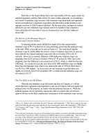
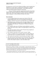
(equipment) or a lot of capital and little labor. In Figure 10.A1, a firm can produce 100
pairs of jeans a day with five different combinations of labor and machines. Combination
a requires seven workers and ten machines; combination b, five workers and fifteen
machines. (To keep output constant, the use of labor must be reduced when the use of
machines is increased. If the use of both were increased, output would rise.)
Curves like the one in Figure 10.A1 are called isoquants. An isoquant curve
(from the Greek words for “same quantity”) is a curve that shows the various technically

efficient combinations of resources that can be use to produce a given level of output.
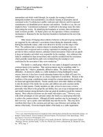
Different output levels have different isoquants. The higher the output level, the higher
the isoquant curve, as shown in Figure 10.A2. For example, an output level of 100 pairs
of jeans can be produced with the resource combinations shown on curve 1Q
1
. An output
level of 150 pairs of jeans requires larger resource combinations, shown on curve 1Q
2
.
To understand how the firm determines its most efficient resource combination,
we must remember that it operates under conditions of diminishing marginal returns. The
firm will always produce in the upward sloping range of its marginal cost curve; and
marginal cost increases because marginal returns decline. Therefore, given a fixed
quantity of one resource as more of another resource is used, the additional output
marginal product, of that resource must diminish.
Then, as each additional worker is eliminated in Figure 10.A1, the number of
machines added to keep output constant at 100 pairs of jeans must rise—and that is just
what happens. Notice that as the firm moves down curve abcde, using fewer and fewer
workers, the curve flattens out. At the same time that the marginal product of machines
diminishes, the marginal product of the remaining workers rises.
Suppose, for instance, that the daily wage of labor is $100, and the daily rental for
a sewing machine is $20. With a daily budget of $600, a firm can employ six workers
and no machines or thirty machines and no workers. Or it can combine labor and
machinery in various ways. It can employ four workers at a total expenditure of $400
and add ten machines at a total expenditure of $200. Curve IC
1
in Figure 10.A3 shows
the various combinations of workers and machines the firm could choose. This kind of
Chapter 10 Production Costs in the
Short Run and Long Run

22
curve is called an isocost curve. An isocost (meaning “same cost”) curve is a curve that
shows the various combinations of resources that can be employed at a given total
expenditure (cost) level and given resource prices.



















We know, then, that the marginal product of resources differs with their level of
use. To determine exactly which combination of resource should be employed to
produce any given output level, however, we need to know not only the marginal

product, but also the prices of labor and capital. The absolute prices of these resources
will determine how much can be produced with any given expenditure. The relative
prices will determine the most efficient combination.
There are different isocost curves for different output levels. The higher the
output, the higher the isocost curve. As long as the prices of labor and capital stay the
same, however, the various isocost curves for different output levels will be parallel to
one another and will have the same downward slope.
Using both isoquant and isocost curves, we can determine the most efficient
resource combination for a given expenditure level. Assuming a firm is on isocost curve
IC
1
in Figure 10.A3 (which represents an expenditure of $600 per day), the most
technically efficient and cost-effective combination of labor and capital will be point a,
three workers and fifteen machines. At point a isocost curve IC
2
is tangent to isoquant

FIGURE 10.A1 Isoquant
A firm can produce one hundred pairs of jeans a day
using any of the various combinations of labor and
machinery shown on this curve. Because of diminishing
marginal returns, more and more machines must be
substituted for each worker who is dropped.

FIGURE 10.A2 Several Isoquants
Different output levels will have different
insoquants. The higher the output level, the
higher the isoquant.