Tài liệu Microeconomics for MBAs 36 pdf

Chapter 10 Production Costs in the
Short Run and Long Run




23
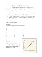
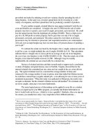
curve IQ
2
. The firm is producing as much as it can 150 pairs of jeans a day with an
expenditure of $600. If it produces the same amount but used more labor on more
capital, it would move to a lower isoquant and a lower output level. A point b on curve
IC
1
, for instance, the firm would lower its production level from 150 to 100 pairs of jeans
per day.
____________________________________
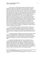
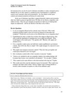
FIGURE 10.A3 Finding the Most Efficient
combination of Resources
Assuming the dial wage of each worker is
$100, and the daily rental on each sewing
machine is $20, an expenditure of $600 per
day will buy any combination of resources
on isocost curve IC
1
. The most cost-
effective combination of labor and capital is
point a, three workers and fifteen machines.
At that point, the isocost curve is just
tangent to isoquant IQ
2

, meaning that the
firm can product 150 pairs of jeans a day. If
the firm chooses any other combination, it
will move to a lower isoquant and a lower
output level. At point b (on isoquant IS
1
), it
will be able to produce only 100 pairs of
jeans a day.

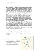
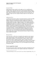
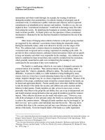
Of course, with increased expenditures, the firm can move to a higher isocost curve. In
figure 10.A4, as the firm’s budget expands, its isocost curve shifts outward from IC
1
to
IC
2
to IC
3
. At the same time, the firm’s most efficient combination of resources increases
from a to b and then to c. As expenditures on resources rise, we can anticipate that
beyond some point the increase in output will not keep pace with the increase in
expenditure; at that point the marginal cost of a pair of jeans will rise.

FIGURE 10.A4 The Effect of Increased
Expenditures on Resources
An increase in the level of expenditures on
resources shifts the isocost curve outward
from IC
1
to IC

2
. The firm’s most efficient
combination of resources shifts from point a
to point c.






Chapter 10 Production Costs in the
Short Run and Long Run




24

PERSPECTIVES: Dealing with the Very Long Run
Economic analysis tends to be restricted to either the short or the long run, for one major reason. For both
periods, costs are known with reasonable precision. In the short run, firms know that beyond some point,
increases in the use of a resource (for example, fertilizer) will bring diminishing marginal returns and rising
marginal costs. They also know that with increased use of all resources, certain economies and
diseconomies of scale can be expected over the long run. Given what is known about the technology of
production and the availability of resources, economists can draw certain conclusions about a firm’s
behavior and the consequences of its actions.
As economists look further and further into the future, however, they can predict less about a firm’s
behavior and its consequences in the marketplace. Less is known about the technology and resources of
the distant future. In the very long run, everything is subject to change—resources themselves, their
availability, and the technology for using them. The very long run is the time period during which the

technology of production and the availability of resources can change because if invention, innovation, and
discovery of new technologies and resources.
By definition, the very long run is, to a significant degree, unpredictable. Firms cannot know today how
to make use of unspecified future advances in technology. A hundred years ago firms had little idea how
important lasers, satellites, airplanes, and computers would be to today’s economy. Indeed, many products
taken for granted today were invented or discovered quite by accident. Edison developed the phonograph
while attempting to invent the light bulb. John Rock developed the birth control pill while studying
penicillin, Charles Goodyear’s development of vulcanization, and Wilhelm Roentgen’s invention of the x-
ray—all were accidents. All had economic consequences that could not have been predicted.
Not all inventions or innovations are accidental, and we can know something about the very long run.
Firms have some idea of the value of investments in research and development. Research on substitute
resources can yield improvements in productivity that translate into cost reductions. Research on new
product designs will yield more attractive and useful products. There will be failures as well—research
projects that accomplish little or nothing—but over time, the rewards of research and development can
exc eed the costs.
Because of the risks involved in research and development, some firms may be expected to fail. In the
very long run, they will not be able to keep up with the competition in product design and productivity.
The will not adjust sufficiently to changes in the market and will suffer losses. The computer industry
provides many examples of firms that tried to build a better machine, but could not keep pace with the
rapid technological advances of competitors.
Proponents of a planned economy see the uncertainty of the very long run as an argument for
government direction of the nation’s development. They stress that competitors often do not know what
other firms are doing. Therefore they need guidance in the form of government subsidies and tax penalties
to ensure that the nation’s long-term goals are achieved.
Proponents of the market system agree that it is difficult to look ahead to the very long run, but they see
the uncertainties as an argument for keeping production decisions in the hands of firms. Private firms have
the economic incentive of profit to stay alert to changes in market conditions, and they can respond quickly
to changes in technology and resources. Government control might slow the adjustment process.

CHAPTER 11

Firm Production under Idealized
Competitive Conditions

Economists understand by the term market, not any particular market place in which things
are bought and sold, but the whole of any region in which buyers and sellers are in such free
intercourse with one another that the prices of the same goods tend to equality, easily and
quickly.
Augustin Cournot
receding chapters dealt separately with the two sides of markets, consumers and
producers. We devised graphic means of representing consumer preferences (the
demand curve) and producer costs (average and marginal cost curves). This chapter
brings demand and cost analysis together in order to examine the way in which individual
firms react to consumer demand in competitive markets. Our focus will be on a highly
competitive market structure called perfect competition. We will investigate an intriguing
question: at the limit, how much can competitive markets contribute to consumer welfare?
We will not attempt to give a full description of a real-world competitive market
setting. Because markets are so diverse, such a description would probably not be very
useful. Our aim is rather to devise a theoretical framework that will enable us to think about
how markets work in general, as a constructive behavioral force. Although our model cannot
tell much that is specific about real-world markets, it will provide a basis for predicting the
general direction of changes in market prices and output. Through its analysis, we should
gain a deeper understanding of the meaning of market efficiency.
Perfect competition is only one of four basic market structures. The other three, and
the detrimental effects of their restrictions on competition, are the subjects of following
chapters.

The Four Market Structures

Markets can be divided into four basic categories, based on the degree of competition that
prevails within them that is, on how strenuously participants attempt to outdo, and avoid
being outdone by, their rivals. The most competitive of the four market structures is perfect
competition.

Perfect Competition
As we stressed much earlier in the book, perfect competition represents an ideal degree of
competition. Perfect competition can be recognized by the following characteristics:
P
Chapter 11 Firm Production under Idealized
Competitive Conditions





1. There are many producers in the market, no one of which is large enough to
affect the going market price for the product. All producers are price takers,
as opposed to price searchers or price makers (see the Perspective on the
subject below).
2. All producers sell a homogeneous product, meaning that the goods of one
producer are indistinguishable from those of all others. Consumers are fully
knowledgeable about the prices charged by different producers and are totally
indifferent as to which producer they buy from.
3. Producers enjoy complete freedom of entry into and exit from the market—
that is, entry and exit costs are minimal, although not completely absent.
4. There are many consumers in the market, no one of whom is powerful enough
to affect the market price of the product. Like producers, consumers are price
takers.
As we have seen before, the demand curve facing the individual perfect competitor is

not the same as the demand curve faced by all producers. The market demand curve slopes
downward, as shown in Figure 11.1(a). The demand curve facing an individual producer
price taker is horizontal, as in Figure 11.1(b). This horizontal demand curve is perfectly
elastic. That is, the individual firm cannot raise its price even slightly above the going
market price without losing all its customers to the numerous other producers in the market
or to other producers waiting for an opportunity to enter the market. On the other hand, the
individual firm can sell all it wishes at the going market price. Hence it has no reason to
offer its output at a lower price. The markets for wheat and for integrated computer circuits,
or computer chips, are both good examples of real-world markets that come close to perfect
competition.

Pure Monopoly
Pure monopoly: A single seller of a product for which there are no close substitutes.
Protected from competition by barriers to entry into the market. The barriers to entry into the
monopolist’s market will be described in the next chapter. For now, we will simply note that
because the monopolistic firm does not have to worry about competitors undercutting its
price, it can raise its price without fear that customers will move to other producers of the
same product or similar products. All the pure monopolist has to worry about is losing
customers to producers of distantly related products.
Since the monopolist is the only producer of a particular good, the downward-sloping
market demand curve [Figure 11.1(a)] is its individual demand curve. Unlike the perfect
competitor, the monopolistic firm can raise its price and sell less, or lower its price and sell
more. The critical task of the pure monopolist is to determine the one price-quantity
combination of all price-quantity combinations on its demand curve that maximizes its
profits. In this sense the pure monopolist is a price searcher. The best (but not perfect) real-
world examples of a pure monopoly are regulated electric-power companies, which dominate
in given geographical areas, and the government’s first-class postal system.
Chapter 11 Firm Production under Idealized
Competitive Conditions

FIGURE 11.1 Demand Curve Faced by Perfect Competitors
The market demand for a product part (a) is always downward sloping. The perfect competitor is on a
horizontal, or perfectly elastic, demand curve [part (b)]. It cannot raise its price above the market price even
slightly without losing its customers to other producers.


Monopolistic Competition
Monopolistic competition is a market composed of a number of producers whose products
are differentiated and who face highly elastic, but not perfectly elastic, demand curves.
A monopolistically competitive market can be recognized by the following
characteristics:
1. There are a number of competitors, producing slightly different products.
2. Advertising and other forms of nonprice competition are prevalent.
3. Entry into the market is not barred but is restricted by modest entry costs, mainly
overhead.

4. Because of the existence of close substitutes, customers can turn to other
producers if a monopolistically competitive firm raises its price. Because of brand
loyalty, the monopolistic competitor’s demand curve still slopes downward; but it is
fairly elastic [see Figure 11.2).
The market for textbooks is a good example of monopolistic competition. Most subjects are
covered by two or three dozen textbooks, differing from one another in content, style of
presentation, and design.
Chapter 11 Firm Production under Idealized
Competitive Conditions





PERSPECTIVE: Price Takers and Price Searchers
Perfect competition is an extreme degree of competition, so much so that many students are understandably
concerned about its relevance. They often ask, “If there are few market structures that even closely approximate
perfect competition, why bother to study it?” The question is a good one and not altogether easy to answer.
There are few markets that come close to having numerous producers of an identical product with complete
freedom of entry and exit. Markets for agricultural commodities and for stocks and bonds are probably the
closet markets we have to perfect competition, but still the products are not always completely identical, and
entry and exit costs abound in most markets. Even wheat sold by a Kansas wheat farmer us not always viewed
the same as wheat sold by a Texas wheat farmer.
How can sense be made of perfect competition? The answer is remarkably simple. We know that under the
conditions of competition specified, certain results follow. We can logically (with the use of graphs and
mathematics) derive them, and the results are developed in this and the following chapter. One conclusion
drawn is that in perfect competition each firm will extend production until the marginal cost of producing the
last unit equals the price paid by the consumer. That conclusion necessarily follows. As we will see, it is
mathematically valid. The strict (extreme) assumptions about the nature of perfect competition assure that.
The demanding conditions for perfect competition are rarely met. We nevertheless cannot conclude that

under less demanding competitive conditions, competitive results would not be observed. [see the Perspectives
on contestable markets on page 240.) For example, it may be that the number of producers is not “numerous”
that the products sold by all producers are not completely “identical,” and that there are costs to moving in and
out of markets. Nonetheless, individual producers may act as if the conditions of perfect competition are met.
Individual producers may still act as if they have no control over market price or that there are so many other
actual or potential producers that it is best to think in terms of the other producers being numerous”—in which
case many of the predicted results of perfect competition may be still observed in the less-than-perfect markets.
For these reasons, many economists often talk not about perfect competitors but about price takers (who may
or may not fit exactly the description of perfect competitors). Price takers are sellers who do not believe they
can control the market price by varying their own production levels. They simply observe the market price and
either accept it (and produce accordingly, to the point where marginal cost and marginal revenue and price are
equal) or reject it (and go into some other business). The price taker is someone who acts as if his or her demand
curve is horizontal (perfectly elastic, more or less). He or she is therefore someone who assumes the marginal
revenue on each unit sold is constant (and equal to the price)—and that the marginal revenue curve is horizontal
and the same as the firm’s demand curve.
The price searcher stands in contrast to the price taker. Price searchers are sellers who have some control
over the market price. Price searchers have monopoly power due to the fact that they can alter production and
thereby market supply sufficiently to change the price. The individual price searcher’s task is not simply to
accept or reject the current market price, but (like the monopolist) to “search” through the various price-quantity
combinations on his or her downward sloping demand curve with the intent upon maximizing profits. As we
will see i
n the following chapter, the marginal revenue and demand curves of the price searcher are no longer the
same. (Exactly where the monopolist’s marginal revenue curve lies in relation to the demand curve will be
discussed in detail in the next chapter).

Chapter 11 Firm Production under Idealized
Competitive Conditions

________________________________________
FIGURE 11.2 Demand Curve Faced by a
Monopolistic Competitor
Because the product sold by the monopolistically
competitive firm is slightly different from the
products sold by competing producers, the firm
faces a highly elastic, but not perfectly elastic,
demand curve.



Oligopoly
An oligopoly is a market composed of only a handful of dominant producers—as few as
two—whose pricing decisions are interdependent. Oligopolists may produce either an
identical product (like steel) or highly differentiated products (like automobiles). Generally
the barriers to entry into the market are considerable, but the critical characteristic of
oligopolistic firms is that their pricing decisions are interdependent. That is, the pricing
decisions of any one firm can substantially affect the sales of the others. Therefore, each
firm must monitor and respond to the pricing and production decisions of the other firms in
the industry. The importance of this characteristic will become clear in a following chapter.
Table 11.1 summaries the characteristics of the four market structures.

The Perfect Competitor’s Production Decision
As we learned earlier, the market price in a perfectly competitive market is determined by the
intersection of the supply and demand curves. If the price is above the equilibrium price
level, a surplus will develop forcing competitors to lower their prices. If the price is below
equilibrium, a shortage will emerge, pushing the price upward [see Figure 11.3(a)]. Given a

market price over which it has no control, how much will the individual perfect competitor
produce?

The Production Rule: MC = MR
Suppose the price in the perfectly competitive market for computer chips $5 (P
1
in Figure
11.3). For each individual competitor, the market price is given, that is, cannot be changed.
It must be either accepted or rejected. If the firm rejects the price, however, it must shut
down. If it raises its price even slightly above the market level, its customers will move to
other competitors.) Demand, then, is horizontal at $5.
Chapter 11 Firm Production under Idealized
Competitive Conditions





Table 11.1 Characteristics of the Four Market Structures.

Number of
Firms
Freedom of
Entry
Type of Product
Example
Perfect competition Many Very easy Homogeneous Wheat,
Computers,
and
Gold

Pure monopoly One Barred Single product Public utilities
and
Postal service
Monopolistic com-
petition
Many Relatively easy Differentiated Pens,
Books,
Paper, and
Clothing
Oligopoly Few Difficult Either standardized
or differentiated
Steel,
Light bulbs,
Cereal, and
Autos
_____________________________________________________________________

The firm’s perfectly elastic horizontal demand curve is illustrated on the right side of
Figure 11.3. This horizontal demand curve is also the firm’s marginal revenue curve,
because marginal revenue is defined as the additional revenue acquired from selling one
additional unit. Because each computer chip can be sold at a constant price of $5, the
additional, or marginal, revenue acquired from selling an additional unit must be constant at
$5.
Because profit equals total revenue minus total cost (profit = TR = TC), the profit-
maximizing firm will produce any unit for which marginal revenue exceeds marginal cost.
Thus the profit-maximizing firm in Figure 11.3(b) will produce and sell q
1
units, the quantity
at which marginal revenue equals marginal cost (MR = MC). Up to q
1

, marginal revenue is
greater than marginal cost. Beyond q
1
, all additional computer chips are unprofitable: the
additional cost of producing them is greater than the additional revenue acquired [with the
small “q” being used to remind you that the output individual producer in Figure 11.3(b) is a
small fraction of the output for the market, designated by a capital “Q” in Figure 11.3 (a)].

Changes in Market Price
The perfectly competitive firm produces where MC = MR, both of which are equal to price.
Thus the amount the firm produces depends on market price. As long as market demand
remains constant, the individual firm’s demand, and its price, will also remain constant. If
market demand and price increase, however, the individual firm’s demand and price will also
increase.
Chapter 11 Firm Production under Idealized
Competitive Conditions

FIGURE 11.3 The Perfect Competitor’s Production Decision
The perfect competitor’s price is determined by market supply and demand [part (a)]. As long as
marginal revenue (MR), which equals market price, exceeds marginal cost (MC), the perfect
competitor will expand production [part (b)]. The profit-maximizing production level is the point
at which marginal cost equals marginal revenue (price).













FIGURE 11.4 Change in the Perfect Competitor’s Market Price
If the market demand rises from D
1
to D
3
[part (a)], the price will rise with it, from P
1
to P
3
. As a

result, the perfectly competitive firm’s demand curve will rise, from d1 to d3 [part (b)].


Chapter 11 Firm Production under Idealized
Competitive Conditions





Figure 11.4 (above) shows how the shift occurs. The original market demand of D
1

leads to a market price of P
1
[part (a)], which is translated into the individual firm’s demand,
d
1
[part (b)]. The firm maximizes profit by equating marginal cost with marginal revenue,
which is equal to d
1
, at an output level of q
1
.
1

An increase in market demand to D
2
leads to the higher price P
2

and a higher
individual demand curve, d
2
. At this higher price, which equals marginal revenue, the perfect
competitor can support a higher marginal cost. The firm will expand production from q
1
to
q
2
. In the same way, an even greater market demand, D
3
, will lead to even higher output, q
3
,
by the individual competitor.
Why does the market supply curve slope upward and to the right? The answer lies in
the upward-sloping marginal cost curves confronted by individual firms. (The market supply
curve is obtained by horizontally adding the supply curves of individual firms.) The
individual firm’s marginal cost curves slope upward because of diminishing (marginal)
returns, a technological fact of the production process.

Maximizing Short-Run Profits
Can perfect competitors make an economic profit? The answer is yes, at least in the short
run. To see this point, we must incorporate the average and marginal cost curves developed
in the last chapter into our graph of the perfect competitor’s demand curve, as in Figure
11.5(b). [Figure 11.5(a) shows the market supply and demand curves.) As before, the
producer maximizes profits by equating marginal cost with price, rather than by looking at
average cost. That is exactly what the perfect competitor does. The firm produces q
2

computer chips because that is the point at which marginal revenue curve (which equals the
firm’s demand curve crosses the marginal cost curve. At that intersection, marginal revenue
of the last unit sold equals its marginal cost. If less were produced that q
1
, the marginal cost
would be less than the marginal revenue, and profits would be lost. Similarly, by producing
anything more than q
2
, the firm incurs more additional costs (as indicated by the marginal

1
To prove this statement, first we note that
QPTR=
Then we define short-run total cost to be a function of output:
SRTC = C (Q)
Next, we define profits π to be
)Q(CQPSRTCTR −=−=π
Differentiating with respect to Q and equating with 0, we then obtain
dQ
)Q(dC
P
0
dQ
)Q(dC
P
dQ
d
=
=−=
π

Since
dQ
)Q(dC
= SRMC, profits are maximized when SRMC P= .