Tài liệu Phần mềm xác định radio P6 docx

6
The Digital Front End – Bridge
Between RF and Baseband
Processing
Tim Hentschel and Gerhard Fettweis
Technische Universita
¨
t Dresden
6.1 Introduction
6.1.1 The Front End of a Digital Transceiver
The first question that might arise is: What is the digital front end? The notion of the digital
front end (DFE) has been introduced by the author in several publications (e.g. [13]). None-
theless it is useful to introduce the concept of the DFE at the beginning of this chapter.
Several candidate receiver and transmitter schemes have been presented by Beach et al. in
Chapter 2. They all have in common that they are different from the so-called ideal software
radio insofar as the signal has to undergo some signal processing steps before the baseband
processing is performed on a software programmable digital signal processor (DSP). These
signal processing stages between antenna and DSP can be grouped and called the front end of
the transceiver.
Historically, the notion of a front end was applied to the very part of a receiver that was
mounted at or near the antenna. It delivered a signal at an intermediate frequency which was
carried along a wire to the back end. The back end was possibly placed apart from the
antenna. In the current context the notion of the front end has been undermined a bit and
moreover extended to the transmitter part of a transceiver. The functionality of the front end
can be derived from the characteristics of the signals at its input and output. Figure 6.1 shows
the front end located between the antenna and baseband processing part of a digital receiver.
Its input is fed with an analog wide-band signal comprising several channels of different
services (air interfaces). There are N
i
channels of bandwidth B
i

of the ith service (air inter-
face). Integrating over all services i yields the total bandwidth B of the wide-band signal. It
includes the channel-of-interest that is assumed to be centered at f
c
.
Software Defined Radio
Edited by Walter Tuttlebee
Copyright q 2002 John Wiley & Sons, Ltd
ISBNs: 0-470-84318-7 (Hardback); 0-470-84600-3 (Electronic)
The output of the front end must deliver a digital signal (ready for baseband processing)
with a sample rate determined by the current air interface. This digital signal represents the
channel-of-interest of bandwidth B
i
centered at f
c
¼ 0. Thus, the front end of a digital
receiver must provide a digital signal
† of a certain bandwidth,
† at a certain center frequency, and
† with a certain sample rate.
Hence, the functionalities of the front end of a receiver can be derived from the four empha-
sized words as:
† channelization,
– down-conversion of the channel-of-interest from RF to baseband, and
– filtering (removal of adjacent channel interferers and possibly matched filtering),
† digitization,
† sample-rate conversion, and
† (synchronization).
Should synchronization belong to the front end or not? If the front end is equivalent to what
Meyr et al. [19] call the inner receiver, synchronization is part of the front end. Synchroniza-

tion basically requires two tasks: the estimation of errors (timing, frequency, and phase)
induced by the channel, and their correction. The latter can principally be realized with the
same algorithms and building blocks as the channelization and sample-rate conversion. The
estimation of the errors is extra. In the current context these estimation algorithms should not
be regarded as part of the front end. The emphasis lies on channelization, digitization, and
sample-rate conversion.
Having identified the front end functionalities, the next step is to implement them. The
question arises of where channelization should be implemented, in the analog or digital
domain. As the different architectures in Chapter 2 suggest, some parts of channelization
can be realized in the analog domain and other parts in the digital domain. This leads to
Software Defined Radio: Enabling Technologies152
Figure 6.1 A digital receiver
distinguishing the analog front end (AFE) and the digital front end (DFE) as shown in
Figure 6.2. Thus, the digital front end is part of the front end. It performs front end function-
alities digitally. Together with the analog-to-digital converter it bridges the analog RF- and
IF-processing on one side and the digital baseband processing on the other side.
The same considerations that exist for the receiver are valid for the transmitter of a soft-
ware defined transceiver. In the following, the receiver will be dealt with in most cases. Only
where the transmitter needs special attention will it be mentioned explicitly.
In order to support the idea of software radio, the analog-to-digital interface should be
placed as near to the antenna as possible thus minimizing the AFE. However, this means that
the main channelization parts are performed in the digital domain. Therefore the signal at the
input to the analog-to-digital converter is a wide-band signal comprising several channels, i.e.
the channel-of-interest and several adjacent channel interferers as indicated by the bandwidth
B in Figure 6.1. On the transmitter side the spurious emission requirements must be met by
the digital signal processing and the digital-to-analog converter. Hence, the signal character-
istics are an important issue.
6.1.2 Signal Characteristics
Signal characteristics means what the DFE must cope with (in the receiver) and what it must
fulfill (in the transmitter). This is usually fixed in the standards of the different air interfaces.

These standards describe, e.g. the maximum allowed power of adjacent channel interferers
and blockers at the input of a receiver. From these figures the maximum dynamic range of a
wide-band signal at the input to a software radio receiver can be derived. These specifications
for the major European mobile standards are given in the Appendix to Chapter 2.
The maximum allowed power of adjacent channels increases with the relative distance
between the adjacent channel and the channel-of-interest. Therefore, the dynamic range of a
wide-band signal grows as the number of channels that the signal comprises increases. In
order to limit the dynamic range, the bandwidth of the wide-band signal must be limited. This
is done in the AFE. By this means the dynamic range can be matched to what the analog-to-
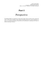
digital converter can cope with. Assuming a fixed filter in the AFE, the total number of
channels inside the wide-band signal depends on the channel bandwidth. This is sketched in
Figure 6.3 for the air interfaces, UMTS (universal mobile telecommunications system), IS-
95, and GSM (global system for mobile communications), assuming a total bandwidth of
B ¼ 5 MHz, and where
d
stands for the minimum required signal-to-noise ratio of the
channel-of-interest which is assumed to be similar for the three air interfaces.
Obviously, a trade-off between total dynamic range and channel bandwidth can be made.
The Digital Front End – Bridge Between RF and Baseband Processing 153
Figure 6.2 The front end of a digital receiver
The smaller the channel bandwidth is, the larger is the number of channels inside a fixed
bandwidth and thus, the larger is the dynamic range of the wide-band signal. This trade-off
has been named the bandwidth dynamic range trade-off [13]. It is important to note that only
the channel-of-interest is to be received. This means that the possibly high dynamic range is
required for the channel-of-interest only. Distortions, e.g. quantization noise of an analog-to-
digital converter, must be limited or avoided only in the channel-of-interest. This property
can be exploited in the DFE resulting in reduced effort, e.g.
1. the noise shaping characteristics of sigma-delta analog-to-digital converters fit this
requirement perfectly [11],
2. filters can be realized as comb filters with low complexity (this is dealt with in

Sections 6.4.1 and 6.5.4).
On the transmitter side the signal characteristics are not as problematic as on the receiver side.
Waveforms and spurious emissions are usually provided in the standards. These figures must
be met, influencing the necessary processing power, the word length, and thus the power
Software Defined Radio: Enabling Technologies154
Figure 6.3 Signal characteristics and the bandwidth dynamic range trade-off (adapted from [13],
q 1999 IEEE)
consumption. However, a critical part is the wide-band AFE of the transmitter. Since there is
no analog narrow-band filter matched to the channel bandwidth, the linearity of the building
blocks, e.g. the power-amplifier, is a crucial figure.
6.1.3 Implementation Issues
In order to implement as many functionalities as possible in the digital domain and thus
provide a means for adapting the radio to different air interfaces, the sample rates at the
analog/digital interface are chosen very high. In fact, they are chosen as high as the ADC and
DAC allow. The algorithms realizing the functionalities of the DFE must be performed at
these high sample rates. As an example, digital down-conversion should be mentioned. As
can be seen in Section 6.3, a digital image rejection mixer requires four real multiplications
per complex signal sample. Assuming a sample rate of 100 million samples per second
(MSps) this yields a multiplication rate of 400 million multiplications per second. This
would occupy a good deal of the processing power of a DSP, however, without really
requiring its flexiblity. Therefore it is not sensible to realize digital down-conversion on a
digital signal processor. The same consideration also holds in principle for channelization and
sample-rate conversion: very high sample rates in connection with signals of high dynamic
range makes the application of digital signal processors questionable. If, moreover, the signal
processing algorithms do not require much flexiblity from the underlying hardware platform
it is not sensible to use a DSP.
A solution to this problem is parameterizable and reconfigurable hardware. Reconfigurable
hardware is hardware whose building blocks can be reconfigured on demand. Field program-
mable gate arrays (FPGAs) belong to this class. Up to now these FPGAs have a long
reconfiguration time compared to the processing speed they offer. Therefore they cannot

be reconfigured dynamically, i.e. while processing. On the other hand, the application in
mobile communications systems is well defined. There is a limited number of algorithms that
must be realized. For that reason hardware structures have been developed that are not as fine-
grained as FPGAs. This means that the building blocks are not as general as in FPGAs but are
much more tailored to the application. This results in reduced effort.
If the granularity of the hardware platform is made even more coarse, the hardware is no
longer reconfigurable but parameterizable. Dedicated building blocks whose functionality is
fixed can be implemented on application specific integrated circuits (ASICs) very efficiently. If
the main parameters are tunable, these ASICs can be employed in software defined radio
transceivers. A simple example is the above-mentioned digital down-conversion. The only
thing that must be tunable is the frequency of the local oscillator. Besides this, the complete
underlying hardware does not need to be changed. This is very efficient as long as digital down-
conversion is required. In a potential operation mode not requiring digital down-conversion of
a software radio, the dedicated hardware block cannot be used and must be regarded as ballast.
However, with respect to the wide-band signal at the output of the analog-to-digital
converter in a digital receiver, it is sensible to assume that the functionalities of the DFE,
namely channelization and sample-rate conversion, are necessary for most air interfaces.
Hence, the idea of dedicated parameterizable hardware blocks promises to be an efficient
solution. Therefore, all considerations and investigations in this chapter are made with respect
to an implementation as reconfigurable hardware.
Hardware and implementation issues are covered in detail in subsequent chapters.
The Digital Front End – Bridge Between RF and Baseband Processing 155
6.2 The Digital Front End
6.2.1 Functionalities of the Digital Front End
From the previous section it can be concluded that the functionalities of the DFE in a receiver
are
† channelization (i.e. down-conversion and filtering), and
† sample-rate conversion.
The functionalities of a receiver DFE are illustrated in Figure 6.4. It should be noted that the
order of the three building blocks (digital down-conversion, SRC, and filtering) is not neces-

sarily as shown in Figure 6.4. This will become clear in the course of the chapter.
Since the DFE should take over as many tasks as possible from the AFE in a software radio,
the functionalities of the DFE are very similar to what has been described in Section 6.1.1 for
the front end in general. The digitized wide-band signal comprises several channels among
which the channel-of-interest is centered at an arbitrary carrier frequency. Channelization is
the functionality that shifts the channel-of-interest to baseband and moreover removes all
adjacent channel interferers by means of digital filtering.
Sample rate conversion (SRC) is a relatively ‘young’ functionality in a digital receiver. In
conventional digital receivers the analog/digital interface has been clocked with a fixed rate
derived from the master clock rate of the air interface that the transceiver was designed for. In
Software Defined Radio: Enabling Technologies156
Figure 6.4 A digital receiver with a digital front end
software radio transceivers there is no isolated target air interface. Therefore the transceiver
must cope with different master clock rates. Moreover, it must be borne in mind that the
terminal and base station run mutually asynchronously and must be synchronized when the
connection is set up.
There are two approaches to overcome these two problems. First, the analog/digital inter-
face can be clocked with a tunable clock. Thus, for all air interfaces the right sampling clock
can be used. Additionally, it is possible to ‘pull’ the tunable oscillator for synchronization
purposes. It is clear that such a tunable oscillator requires considerably more effort than a
fixed one. For that reason designers favour the application of a fixed oscillator. Nonetheless,
the baseband processing requires a signal with a proper sample rate. Hence, sample-rate
conversion is necessary in this case for converting between the fixed clock rate at the
analog/digital interface and the target rate of the respective air interface.
Very often interpolation (e.g. Lagrange interpolation) is regarded as a solution to SRC.
Still, this solution is only sensible in certain applications. The usefulness of conventional
interpolation depends on the signal characteristics. In Section 6.1.1, it has been mentioned
that the wide-band signal at the input of the DFE of a receiver can comprise several channels
beside the channel-of-interest. However, only the channel-of-interest is really wanted. This
fact can be exploited for reducing the effort for SRC (see Section 6.5).

Since both channelization and SRC require filtering, it is possible to combine them. This
can lead to considerable savings. A well-known example is multirate filtering [1]. This is a
concept where filtering and integer factor SRC (e.g. decimation) are realized stepwise on a
cascaded structure comprising several stages of filtering and integer factor SRC. Generally,
this results in both a lower multiplication rate and a lower hardware complexity.
The functionalities of the transmitter part of a DFE are equivalent to those of the receiver
part: the baseband signal to be transmitted is filtered, digitally up-converted, and its sample
rate is matched to the sample rate of the analog/digital interface. Although there are no
adjacent channels to be removed, filtering is necessary for symbol forming and in order to
fulfill the spurious emissions characteristics dictated by the respective standard. Again,
filtering and SRC can be combined.
There is a strong relationship between digital down-conversion and channel filtering since
they form the functionality channelization. On the other hand, it has been mentioned that
there is also a strong relationship between channel filtering and SRC, e.g. in the case of
multirate filtering. In the main part of this chapter, a separate section is dedicated to each of
the three, digital down-conversion, channel filtering, and sample-rate conversion. Important
relations between them are dealt with in these sections.
6.2.2 The Digital Front End in Mobile Terminals and Base Stations
The great issue of mobile terminals is power consumption. Everything else is less important.
Power consumption is the alpha and the omega of mobile terminal design. On the other hand,
mobile terminals usually must only process one channel at a time. This fact enables the
application of efficient solutions for channelization and SRC that are based on the multirate
filtering concept.
In contrast to this there are no restrictions regarding power consumption in base stations
besides basic environmental aspects. Still, in base stations several channels must be processed
in parallel.
The Digital Front End – Bridge Between RF and Baseband Processing 157
This fundamental difference between mobile terminals and base stations must be kept in
mind when investigating and evaluating algorithms and potential solutions.
6.3 Digital Up- and Down-Conversion

6.3.1 Initial Thoughts
The notion of up- and down-conversion stands for a shift of a signal towards higher or lower
frequencies, respectively. This can be achieved by multiplying the signal
x
a
ðtÞ with a complex
rotating phasor which results in
x
b
ðtÞ¼x
a
ðtÞe
j2
p
f
c
t
ð1Þ
where f
c
stands for the frequency shift. Often f
c
is called the carrier frequency to which a
baseband signal is up-converted, or from which a band-pass signal is down-converted.
However, in this case f
c
would have to be positive. Regarding it as a frequency shift enables
us to use positive and negative values for f
c
.

The real and imaginary parts of a complex signal are also called the in-phase and the
quadrature-phase components, respectively.
Digital up- and down-conversion is the digital equivalent of Equation (1). This means that
both the signals and the complex phasor are represented by quantized samples (quantization
issues are not covered in this chapter). Introducing a sampling period T, that fulfills the
sampling theorem, digital up- and down-conversion can be written as
x
b
ðkTÞ¼x
a
ðkTÞe
j2
p
f
c
kT
ð2Þ
Assuming perfect analog-to-digital or digital-to-analog conversion, respectively,
Equations (1) and (2) are equivalent.
Depending on the sign of f
c
, up- or down-conversion results. Thus, it is sufficient to deal
with one of the two. Only digital down-conversion is discussed in the sequel.
It should be noted that real up- and down-conversion is also possible and indeed very
common, i.e. multiplying the signal with a sine or cosine function instead of the complex
exponential of Equations (1) and (2). However, real up- and down-conversion is a special
case of complex up- and down-conversion and is therefore not discussed separately in this
chapter.
6.3.2 Theoretical Aspects
In order to understand the task of digital down-conversion, it is useful to consider the

complete signal processing chain of up-conversion in the transmitter, transmission, and
final down-conversion in the receiver. It is assumed that the received signal is down-
converted twice. First the complete receive band is down-converted in the AFE. This is
followed by filtering. The processed signal is again down-converted in the DFE. This is
sketched in Figure 6.5.
For the discussion it is assumed that there are no distortions due to the channel, however, it
introduces adjacent channel interferers. Thus, the received signal x
Rx
ðtÞ is equal to the
transmitted signal x
Tx
ðtÞ plus adjacent channel interferers aðtÞ:
Software Defined Radio: Enabling Technologies158
x
Rx
ðtÞ¼x
Tx
ðtÞþaðtÞ
¼ Re
x
Tx;BB
ðtÞe
j2
p
f
c
t
no
þ aðtÞð3Þ
¼

1
2
x
Tx;BB
ðtÞe
j2
p
f
c
t
þ x
Ã
Tx;BB
ðtÞ e
ÿj2
p
f
c
t

þ aðtÞð4Þ
where
x
Tx;BB
ðtÞ is the complex baseband signal to be transmitted. f
c
denotes the carrier
frequency and
x
Ã

the conjugate complex of x. From Equation (4) it can be concluded that
the received signal comprises two components besides the adjacent channel interferers: one
centered at f
c
and another centered at ÿf
c
. The first comprises the signal-of-interest x
Tx;BB
ðtÞ.
It lies anywhere in the frequency band of bandwidth B which comprises several frequency
divided channels, i.e. the channel-of-interest plus adjacent channel interferers. This band is
selected by a receive band-pass filter. The arrangement of the channel-of-interest (i.e. the
signal x
Rx
ðtÞ) in the receive frequency band is sketched in Figure 6.6.
As mentioned above the analog front end performs down-conversion of the complete
receive frequency band of bandwidth B. Inside this frequency band lies the signal-of-interest
x
Tx;BB
ðtÞ which should finally be down-converted to baseband. The following signal is
produced at the output of the analog down-converter when down-converting by f
1
. For
reasons of simplicity of the derivation we shall limit f
1
to f
1
, f
c
.

x
Rx;IF
ðtÞ¼x
Rx
ðtÞe
ÿj2
p
f
1
t
ð5Þ
¼

1
2
x
Tx;BB
ðtÞ e
j2
p
ðf
c
ÿf
1
Þt
þ x
Ã
Tx;BB
ðtÞ e
ÿj2

p
ðf
c
þf
1
Þt

þ a
filt
ðtÞe
ÿj2
p
f
1
t
ð6Þ
where a
filt
ðtÞ denotes all adjacent channel interferers inside the receive bandwidth B. The
interesting signal component is centered at the intermediate frequency (IF)
The Digital Front End – Bridge Between RF and Baseband Processing 159
Figure 6.5 The signal processing chain of up-conversion, transmission, and final down-conversion of
a signal (LO stands for local oscillator)
f
IF
¼ f
c
ÿ f
1
ð7Þ

It is enclosed by several adjacent channel interferers. A second signal component lies 2f
c
apart from the first (sketched in Figure 6.7).
The latter is of no interest; moreover, it can cause aliasing in the analog-to-digital conver-
sion process. Therefore it is removed by low-pass (or band-pass) filtering. Thus, the digitized
signal is:
x
dig;IF
ðkTÞ¼
1
2
x
Tx;BB
ðkTÞe
j2
p
f
IF
kT
þ a
dig
ðkTÞð8Þ
where
a
dig
ðkTÞ stands for the remaining adjacent channels after down-conversion, anti-alias-
ing filtering, and digitization. T is the sampling period that must be small enough to fulfill the
sampling theorem. In general the digital IF signal is a complex signal; the interesting signal
component is centered at f
IF

.
The objective of digital down-conversion is to shift this interesting component from the
carrier frequency f
IF
down to baseband. By inspection of Equation (8) it can be found that
down-conversion can be achieved by multiplying the received signal with a respective expo-
nential function:
Software Defined Radio: Enabling Technologies160
Figure 6.6 Position of the channel-of-interest in the receive frequency band of bandwidth B
Figure 6.7 Position of the channel-of-interest at IF
x
dig;BB
ðkTÞ¼x
dig;IF
ðkTÞe
ÿj2
p
f
IF
kT
ð9Þ
¼
1
2
x
Tx;BB
ðkTÞþa
dig
ðkTÞe
ÿj2

p
f
IF
kT
ð10Þ
This yields a sampled version of the transmitted signal
x
Tx;BB
ðtÞ scaled with a factor 1/2. It is
sketched in Figure 6.8. The adjacent channel interferers can be removed with a channelization
filter (see Section 6.4).
It should be noted that in reality the oscillators of transmitter and receiver are not synchro-
nized. Therefore, down-conversion in the receiver yields a signal with phase offset and
frequency offset that must be corrected. The aim of the derivation in this section was to
show what happens with the signal in principle in the individual processing stages and not to
discuss all possible imperfections.
6.3.3 Implementation Aspects
In practical applications it is necessary to treat the real- and imaginary part of a complex
signal separately as two individual real signals. Thus, the signal after analog down-conver-
sion comprises the following two components:
Re
x
Rx;IF
ðtÞ

¼ Re x
Rx
ðtÞ e
ÿj2
p

f
1
t
no
¼ x
Rx
ðtÞ cos 2
p
f
1
t

ð11Þ
Im x
Rx;IF
ðtÞ

¼ Im x
Rx
ðtÞ e
ÿj2
p
f
1
t
no
¼ÿx
Rx
ðtÞ sin 2
p

f
1
t

ð12Þ
It can be concluded that analog down-conversion can be implemented by means of multi-
plying the received real signal by a cosine signal and a sine signal. The real part of the
complex IF signal (also called the in-phase component) is obtained by multiplying the
The Digital Front End – Bridge Between RF and Baseband Processing 161
Figure 6.8 Channel-of-interest at baseband (result of low-pass filtering of the signal of Figure 6.7
followed by digital down-conversion)
received signal with a cosine signal; the imaginary part of the complex IF signal (also called
the quadrature-phase component) is obtained by multiplying the received signal with a sine
signal.
From Equation (8) it can be concluded that the input signal to the digital down-converter is
in principle a complex signal. Hence, the digital down-conversion described by Equation (9)
requires a complex multiplication. Since the complex signals are only available in the form of
their real and imaginary parts, the complex multiplication of the digital down-conversion
requires four real multiplications. By separating the real and imaginary parts of Equation (9),
we have
Re
x
dig;BB
ðkTÞ
no
¼ Re x
dig;IF
ðkTÞ
no
cos 2

p
f
IF
kT

þIm
x
dig;IF
ðkTÞ
no
sin 2
p
f
IF
kT

ð13Þ
Im
x
dig;BB
ðkTÞ
no
¼ Im x
dig;IF
ðkTÞ
no
cos 2
p
f
IF

kT

ÿRe
x
dig;IF
ðkTÞ
no
sin 2
p
f
IF
kT

ð14Þ
This can be regarded as a direct implementation of digital down-conversion. It is sketched in
Figure 6.9.
There are two special cases:
1. When the signal
x
dig;IF
ðkTÞ is real, it is Im x
dig;IF
ðkTÞ
no
¼ 0. Hence, digital down-conver-
sion can be realized by means of two real multiplications in this case.
2. When applying the above results to up-conversion, it is often sufficient to keep the real part
Software Defined Radio: Enabling Technologies162
Figure 6.9 Direct realization of digital down-conversion
of the up-converted signal. Thus, only Equation (13) must be solved resulting in an effort

of two real multiplications and one addition per signal sample.
The samples of the discrete-time cosine and sine functions in Figure 6.9 are usually stored
in a look-up table. The ROM table can simply be addressed by the output signal of an
overflowing phase accumulator representing the linearly rising argument ð2
p
f
IF
kTÞ of the
cosine and sine functions. Requiring a resolution of n bits, the look-up table has a size of
approximately 2
n
 n bits which together with the four general purpose multipliers results in
large chip area, high power consumption, and considerable costs [18].
The large look-up table can be avoided by generating the samples of the digital sine and
cosine functions with an infinite length impulse response (IIR) oscillator. It is an IIR filter
with a transfer function that has a complex or conjugate complex pole on the unit circle [5].
Another way to generate the sine and cosine samples without the need for a large look-up
table is the CORDIC algorithm (CORDIC stands for COordinate Rotation Digital Computer).
The great advantage of the CORDIC algorithm is that it not only substitutes the large look-up
table but also the required four multipliers. This is possible since the CORDIC algorithm can
be used to perform a rotation of the complex phase of a complex number. Interpreting the
samples of the complex signal
x
dig;IF
ðkTÞ as these complex numbers, and rotating the phase of
these samples according to ð2
p
f
IF
kTÞ, the CORDIC algorithm directly performs the digital

up- or down-conversion without the need for explicit multipliers.
6.3.4 The CORDIC Algorithm
The CORDIC algorithm was developed by Volder [25] in 1959 for converting between
cartesian and polar coordinates. It is an iterative algorithm that solely requires shift, add,
and subtract operations. In the circular rotation mode, the CORDIC calculates the cartesian
coordinates of a vector which is rotated by an arbitrary angle.
To rotate the vector
v
0
¼ e
j
f
ð15Þ
by an angle D
f
, v
0
is multiplied by the corresponding complex rotating phasor
v ¼ v
0
·e
jD
f
ð16Þ
The real and imaginary parts of
v are calculated individually:
Re
v
fg
¼ Re v

0
fg
cosðD
f
ÞÿIm v
0
fg
sinðD
f
Þð17Þ
Im
v
fg
¼ Im v
0
fg
cosðD
f
ÞþRe v
0
fg
sinðD
f
Þð18Þ
Rearranging yields
Re v
fg
cosðD
f
Þ

¼ Re
v
0
fg
ÿ Im
v
0
fg
tanðD
f
Þ; jD
f
j Ó
1
2
p
;
3
2
p
; …


ð19Þ
Im v
fg
cosðD
f
Þ
¼ Im

v
0
fg
þ Re
v
0
fg
tanðD
f
Þ; jD
f
j Ó
1
2
p
;
3
2
p
; …


ð20Þ
The Digital Front End – Bridge Between RF and Baseband Processing 163
Note that only the tangent of the angle D
f
must be known to achieve the desired rotation. The
rotated vector is scaled by the factor 1= cosðD
f
Þ.

For many applications it is too costly to realize the two multiplications of Equations (19)
and (20). The idea of the CORDIC algorithm is to perform the desired rotation by means of
elementary rotations of decreasing size, thus iteratively approaching the exact rotation by D
f
.
By choosing the elementary rotation angles as tanðD
f
i
Þ¼^1=2
i
, the multiplications of
Equations (19) and (20) can be replaced by simple shift operations.
D
f
i
¼ ^ arctan 2
ÿi

; i ¼ 0; 1; 2; … ð21Þ
Consequently, in order to rotate a vector
v
0
by an angle D
f
¼ z
0
with jD
f
j ,
p

=2, the
CORDIC algorithm performs a sequence of successively decreasing elementary rotations
with the basic rotation angles D
f
i
¼ ^ arctanð2
ÿi
Þ for i ¼ 0; 1; …; n ÿ 1. The limitation of
D
f
is necessary to ensure uniqueness of the elementary rotation angles. Finally, the iterative
process yields the cartesian coordinates of the rotated vector
v
n
% v. The resulting iterative
process can be described by the following equations for i ¼ 0; 1; …; n ÿ 1:
x
iþ1
¼ x
i
ÿ d
i
y
i
2
ÿi
ð22Þ
y
iþ1
¼ y

i
þ d
i
x
i
2
ÿi
ð23Þ
z
iþ1
¼ z
i
ÿ d
i
arctanð2
ÿi
Þð24Þ
where
x
0
¼ Re v
0
fg
ð25Þ
y
0
¼ Im v
0
fg
ð26Þ

x
n
¼ Re v
n
fg
ð27Þ
y
n
¼ Im v
n
fg
ð28Þ
The figure
d
i
¼
ÿ1ifz
i
, 0
þ1 otherwise

ð29Þ
defines the direction of each elementary rotation. After n iterations the CORDIC iteration
results in
x
n
% A
n
x
0

cosðz
0
Þÿy
0
sinðz
0
Þ

¼ Re A
n
v
0
e
jz
0
no
ð30Þ
y
n
% A
n
y
0
cosðz
0
Þþx
0
sinðz
0
Þ


¼ Im A
n
v
0
e
jz
0
no
ð31Þ
z
n
% 0 ð32Þ
where
Software Defined Radio: Enabling Technologies164
A
n
¼
Y
nÿ1
i¼0
ffiffiffiffiffiffiffiffiffiffi
1 þ 2
ÿ2i
p
ð33Þ
is the CORDIC scaling factor which depends on the total number of iterations. Hence, the
result of the CORDIC iteration is a scaled version of the rotated vector.
In order to overcome the restriction regarding jD
f

j an initial rotation by ^
p
=2 can be
performed if necessary before starting the CORDIC iterations. For details see [15,25].
6.3.5 Digital Down-Conversion with the CORDIC Algorithm
Interpreting each complex sample of the signal x
dig;IF
ðkTÞ of Equation (8) as a complex
number
v
0
, and the angle D
f
ðkÞ¼ÿ2
p
f
IF
kT as z
0
, the CORDIC can be used to continuously
rotate the complex phase of the signal
x
dig;IF
ðkTÞ, thus performing digital down-conversion.
Since the CORDIC is an iterative algorithm, it is necessary to implement each of the itera-
tions by its own hardware stage if high-speed applications are the objective. In such pipelined
architectures the invariant elementary rotation angles arctanð 2
ÿi
Þ of Equation (24) can be
hard-wired. The overall hardware effort of such an implementation of the CORDIC algorithm

is approximately that of three multipliers with the respective word length. Hence one multi-
plier and the ROM look-up table of the conventional approach for down-conversion of
Figure 6.9 can be saved with a CORDIC realization. The principle of digital down-conversion
using the CORDIC algorithm is sketched in Figure 6.10.
For further details on digital down-conversion with the CORDIC the reader is referred to
[18] where quantization error bounds and simulation results are given.
6.3.6 Digital Down-Conversion by Subsampling
The starting point is Equation (8):
x
dig;IF
ðkTÞ¼
1
2
x
Tx;BB
ðkTÞe
j2
p
f
IF
kT
þ a
dig
ðkTÞ
The Digital Front End – Bridge Between RF and Baseband Processing 165
Figure 6.10 Principle of digital down-conversion using the CORDIC algorithm
It is assumed that f
1
has been chosen so that the channel-of-interest is located at a fixed
intermediate frequency f

IF
. The channel can be separated from all adjacent channels by means
of complex band-pass filtering (see Section 6.4.2) at this frequency. Since the bandwidth of
this band-pass filter must be variable in software radio applications, it can be a digital filter
that processes the signal directly after digitization. Hence, it delivers the signal
x
dig-filt;IF
ðkTÞ¼
1
2
x
Tx;BB
ðkTÞe
j2
p
f
IF
kT
ð34Þ
that is sketched in Figure 6.11. At this stage it is assumed that the following relation holds:
f
IF
¼
n
M
1
T
; n ¼ 1; 2; …; M ÿ 1 ð35Þ
i.e. the intermediate frequency is an integer multiple of a certain fraction of the sample rate.
This can easily be achieved since the IF is fixed in most practically relevant systems. As to the

sample rate, the advantage of having a fixed rate has been discussed in Section 6.2.1. Thus,
the ratio of Equation (35) is a parameter that can be specified once in the system design phase.
Substituting Equation (35) in Equation (34) yields
x
dig-filt;IF
ðkTÞ¼
1
2
x
Tx;BB
ðkTÞe
j2
p
ðn=MÞk
ð36Þ
Decimating (i.e. subsampling) the signal
x
dig-filt;IF
ðkTÞ by M eventually leads to
x
dig-filt;IF
ðkMTÞ¼
1
2
x
Tx;BB
ðkMTÞe
j2
p
ðnM=MÞk

ð37Þ
¼
1
2
x
Tx;BB
ðkMTÞð38Þ
which is equivalent to the transmitted baseband signal scaled by 1/2 and with sampling period
MT, supposing that the sampling period MT is short enough to represent the signal, i.e. to
fulfill the sampling theorem (see Figure 6.12). A structure for down-conversion by subsam-
pling is sketched in Figure 6.13.
This process of digital down-conversion is called harmonic subsampling or integer-band
decimation [1]. The equivalent for up-conversion is called integer-band interpolation.Itis
based on up-sampling (see Section 6.5) followed by band-pass filtering [1].
Software Defined Radio: Enabling Technologies166
Figure 6.11 Digitally filtered IF signal (filter bandwidth equals channel bandwidth)
Both methods, integer-band decimation and interpolation are pure sampling processes and
thus, do not require any operation. Still, they do require band-pass filtering, before down-
sampling in the case of down-conversion, and after up-sampling in the case of up-conversion,
respectively. It is the functionality of channel filtering that must be properly combined with
up- or down-sampling in order to have the up- or down-conversion effect. This is discussed in
detail in Section 6.5.
6.4 Channel Filtering
6.4.1 Low-Pass Filtering after Digital Down-Conversion
6.4.1.1 Direct Approach
Figure 6.8 shows the principal channel arrangement in the frequency domain after digital
down-conversion of the channel-of-interest to baseband. This is simply the result of shifting
the right-hand side of Figure 6.7.
Besides the channel-of-interest there are many adjacent channels inside the receive
frequency band of bandwidth B that have been down-converted. In order to select the chan-

nel-of-interest these adjacent channels must be removed with a filter. Since the channel-of-
interest has been down-converted to baseband, a low-pass filter is an appropriate choice.
Infinite length impulse response (IIR) filters are generally avoided due to the nonlinear
phase characteristics which distort the signal. Of course there are cases, especially if the pass-
band is very narrow, where the phase characteristics in the pass-band of the filter can be well
controlled. Still, IIR filters with very narrow pass-band tend to suffer more from stability
The Digital Front End – Bridge Between RF and Baseband Processing 167
Figure 6.12 Result of subsampling the signal of Figure 6.11
Figure 6.13 Principal structure for integer-band decimation (digital down-conversion by subsam-
pling)
problems than those with a wider pass-band. On the other hand IIR filters have very short
group delay. For that reason they might be advantageous in certain applications.
The problems of IIR filters can be avoided when using linear phase filters with finite length
impulse response (FIR). Their great drawback is the generally high order that is necessary to
implement certain filter characteristics compared to the order of an IIR filter with equivalent
performance. For details on digital filter design the reader is referred to the great amount of
literature available in this field.
In order to get some idea of the effort for direct implementation of channel filtering, it is
instructive to learn that for many types of FIR filters (including equiripple FIR filters, FIR
filters based on window designs, and Chebychev FIR filters) the number of coefficients K can
be related to the transition bandwidth Df of the filter and the sample rate f
S
at which it
operates. This proportionality is [1]
K ,
f
S
Df
; Df , f
S

ð39Þ
The transition bandwidth Df is the difference between the cut-off frequency and the lower
edge of the stop band. It can be expressed as a certain fraction of the channel bandwidth.
Thus, it is obvious that the transition bandwidth gets very small compared to the sample rate
f
S
if there is a large number of adjacent channels, i.e. the channel bandwidth itself is very
small compared to f
S
.
Besides the number of coefficients another figure increases with a large number of adjacent
channel interferers: the dynamic range of the signal (see Section 6.1.2). In the case of wide-
band reception of a GSM signal the dynamic range of the signal can easily reach 80 dBand
more. In order to sufficiently attenuate all adjacent channels of such a signal, the processing
word length of the digital filter must be relatively high. A large number of coefficients, a high
coefficient and processing word length, and a high clock rate are indicators for high effort and
costs that are required if the channel filtering functionality is directly implemented by means
of a conventional FIR filter.
As the bandwidth of the digital signal is reduced by filtering there is no reason to keep the
high sample rate that was necessary before filtering. As long as the sampling theorem is
obeyed, the sample rate can be reduced. This results in lower processing rates and thus, lower
effort. Therefore, the high sample rate is usually reduced down to the bit, chip or symbol rate
of the signal after filtering (or a small integer multiple of it). Knowing about the sample rate
reduction after the filtering, it is possible to reduce the filtering effort considerably by
combining filtering and sample rate reduction. This approach is called multirate filtering.
6.4.1.2 Multirate Filtering
The direct approach of implementing the channel filter is a low-pass filter (followed by a
down-sampler). The down-sampler reduces the sample rate according to the bandwidth of the
filtered signal. This is described in the previous section.
For the following discussion it is useful to regard the combination of the filter and the

down-sampler as a system for sample rate reduction (see also Section 6.5). Down-sampling is
a process of sampling. Therefore, it causes aliasing that can be avoided if the signal is
sufficiently band-limited before down-sampling. This band limitation is achieved with
Software Defined Radio: Enabling Technologies168
anti-aliasing filtering. The low-pass filter preceding the down-sampling process, i.e. the
channel filter, acts as an anti-aliasing filter.
Thus, the task of the anti-aliasing filter is to suppress potential aliasing components, i.e.
signal components which would cause distortion when down-sampling the signal. At this
point in the discussion, it is important to note that only the channel-of-interest must not be
distorted. But there is no reason why the adjacent channels should not be distorted. They are
of no interest. Hence, anti-aliasing is only necessary in a possibly small frequency band. In
order to understand the effect of this anti-aliasing property it is useful to introduce the over-
sampling ratio (OSR) of a signal, i.e. the ratio between the sample rate f
S
of the signal, and the
bandwidth b of the signal-of-interest (i.e. the region to be kept free from aliasing).
OSR ¼
f
S
b
ð40Þ
From Figure 6.14 it becomes clear that there are no restrictions as to how the frequencies are
occupied outside the spectrum of the signal-of-interest (e.g. by adjacent channels). This
reflects a general view on oversampling.
The relative bandwidth (compared to the sample rate) of potential aliasing components
(that must be attenuated by the anti-aliasing filter) depends on the OSR after sample rate
reduction. The higher the OSR is, the smaller the pass-band and the stop-bands can be for this
filter. Hence, it can be concluded that a high OSR (after sample rate reduction) allows a wide
transition band Df of the filter and therefore leads to a smaller number of coefficients (see
Equation (39).

Further details on sample rate reduction as a special type of sample rate conversion are
discussed in Section 6.5. The possible savings of multirate filtering are illustrated with the
following example.
The Digital Front End – Bridge Between RF and Baseband Processing 169
Figure 6.14 Illustrating the oversampling ratio (OSR) of a signal
Example 6.4.1
Assuming a sample rate of f
S
¼ 100 MSps, a channel bandwidth of b ¼ 200 kHz, a transition
bandwidth of Df ¼ 40 kHz, and a filter-type specific proportionality factor C, the number of
coefficients of a direct implementation is, with Equation (39),
K
direct
¼ C
f
S
Df
¼ C
100 MHz
40 kHz
% C £ 2500
Further, assuming decimation by 256, only every 256th sample at the output of the filter needs
to be calculated. This results in a multiplication rate (in millions of multiplications per
second, Mmps) of
CðK
direct
Þ¼K
direct
f
S

256
% C £ 980 Mmps
Now a multirate filter with four stages should be applied instead, each stage decimating the
signal by a factor of 4. After these four filters and down-samplers, a fifth filter does the final
filtering (see Figure 6.15). In this case the transition band of the first four filters is equal to the
difference of the sample rate after decimation minus the bandwidth of the channel. This
ensures that potential aliasing components are sufficiently attenuated. Only in the fifth filter
is the transition bandwidth set to 40 kHz. The same filter type as in the previous case is
assumed, hence the same factor C.
K
multirate
¼
X
5
i¼1
K
i
¼ C
X
4
i¼1
100 MHz
4
iÿ1
100 MHz
4
i
ÿ 200 kHz
þ
100 MHz

4
4
40 kHz
"#
% C £ 30:7
Each of the filter stages runs at the lower sampling rate. Thus, the resulting multiplication rate
is
X
5
i¼1
CðK
i
Þ¼
X
4
i¼1
K
i
f
S
4
i
þ K
5
f
S
4
4
Software Defined Radio: Enabling Technologies170
Figure 6.15 Structure of a multirate filter

% C 4
f
S
4
þ 4:1
f
S
16
þ 4:6
f
S
64
þ 8:2
f
S
256
þ 9:8
f
S
256

% C £ 141 Mmps
There is a saving in terms of multiplications per second of a factor 7, while the hardware
effort can be reduced by a factor of 81 in the case of multirate filtering. It should be stressed
that this is an example. The figures can vary considerably in different applications. However,
despite being very special, this example shows the potential of savings that multirate filtering
offers.
Even more savings are possible by employing different filter types for the separate stages in
a multirate filter. The above mentioned factor C is a proportionality factor that was selected
for the direct implementation, e.g. a conventional FIR filter. In the case of multirate filtering it

has been seen that in the first few stages the OSR is very high. This results in relatively large
transition bands. In other words, the stop bands are very narrow. Hence, comb filters suffi-
ciently attenuate these narrow stop-bands. A well-known class of comb filters are cascaded
integrator comb filters (CIC filters) [14]. These filters implement the transfer function
HðzÞ¼
X
Mÿ1
i¼0
z
ÿi
!
R
¼
1 ÿ z
ÿM
1 ÿ z
ÿ1
!
R
without the need for multipliers. M is the sample rate reduction factor and R is called the order
of the CIC filter. Ony adders, subtractors, and registers are needed. Hogenauer [14] states that
these filters generally perform sufficiently for decimating down to four times the Nyquist rate.
Employing these filters in the first three stages of the above example yields K
1
¼ K
2
¼ K
3
¼
0 (i.e. no multiplications required) which would result in a multiplication rate of as low as

C £ 7 Mmps. This is a considerable saving compared to the direct implementation of a low-
pass filter followed by 256 times down-sampling.
A great advantage of CIC filters is that they can be adapted to different rate change factors
by simply choosing M. There is no need to calculate new coefficients or to change the
underlying hardware. Thus, they are a very flexible solution for software defined radio
transceivers. However, as mentioned the OSR after decimation should be at least 4. Thus
the necessary remaining channel-filtering (and possibly matched filtering) can be achieved
with a cascade of two half-band filters, each followed by decimation by 2. Half-band filters
are optimized filters (often conventional FIR filters) for decimation by 2. The half-band filters
do not need to be tunable. Their output sample rate and thus, the signal bandwidth is always
half of that at the input. Hence, by changing the rate-change factor in the CIC filter preceding
the half-band filters, the bandwidth of the overall channel filter is tuned. A final ‘cosmetic’
filtering can be applied to the signal at the lowest sample rate. The respective filter must be
tunable in certain limits, e.g. it must be able to implement root-raised-cosine filters with
different roll-off factors for matched filtering purposes.
For further reading on multirate filtering, the reader is referred to the literature, e.g. [1].
The Digital Front End – Bridge Between RF and Baseband Processing 171
6.4.2 Band-Pass Filtering before Digital Down-Conversion
6.4.2.1 Complex Band-Pass Filtering
Assuming that the channel-of-interest is perfectly selected by the low-pass channel filter with
the discrete-time impulse response h
LP
ðkTÞ (no down-sampling after filtering), it can be
written:
^
x
dig;BB
ðkTÞ¼
X
þ1

i¼ÿ1
h
LP
ðk ÿ iÞTðÞx
dig;BB
ðiTÞð41Þ
where
^
x
dig;BB
ðkTÞ represents the channel-of-interest according to Equation (10):
^
x
dig;BB
ðkTÞ¼
1
2
x
Tx;BB
ðkTÞð42Þ
Substituting Equation (9) into Equation (41) yields
^
x
dig;BB
ðkTÞ¼
X
þ1
i¼ÿ1
h
LP

ðk ÿ iÞTðÞx
dig;IF
ðiTÞe
ÿj2
p
f
IF
iT
ð43Þ
Extracting the factor e
ÿj2
p
f
IF
kT
, we have
^
x
dig;BB
ðkTÞ¼e
ÿj2
p
f
IF
kT
X
þ1
i¼ÿ1
h
LP

ðk ÿ iÞTðÞx
dig;IF
ðiTÞe
j2
p
fIFðkÿiÞT
ð44Þ
¼ e
ÿj2
p
f
IF
kT
X
þ1
i¼ÿ1
h
BP
ðk ÿ iÞTðÞx
dig;IF
ðiTÞð45Þ
with
h
BP
ðkTÞ¼h
LP
ðkTÞ e
j2
p
f

IF
kT
ð46Þ
The latter is the impulse response of the low-pass filter frequency shifted by f
IF
.Itisa
complex band-pass filter. The digitized IF signal
x
dig;IF
ðkTÞ is filtered with this complex
band-pass filter before it is down-converted to baseband. Hence, the down-conversion
followed by low-pass filtering can equivalently be performed by means of complex band-
pass filtering followed by down-conversion.
Both solutions are equivalent in terms of their input–output behavior. However, there are
differences with respect to implementation and realization. Since down-conversion is expli-
citly necessary in both cases, only the filtering operations should be compared.
The length of both impulse responses, the band-pass filter’s and the low-pass filter’s, are
the same. However, the impulse response of the low-pass filter h
LP
ðkTÞ is real. Hence, each
addend of the sum of Equation (41) is a result of multiplying a complex number (i.e. a sample
of the complex signal
x
dig;BB
) with a real number (i.e. a sample of the real impulse response
h
LP
). Consequently, each addend requires two real multiplications, resulting in 2K multi-
plications per output sample if K is the length of the impulse response.
In the case of complex band-pass filtering, Equations (45) and (46) suggest that each

addend is a result of a complex multiplication (i.e. a multiplication of a sample of the complex
signal
x
dig;IF
and the complex impulse response h
BP
) that is equivalent to four real multi-
Software Defined Radio: Enabling Technologies172
plications. Hence, the resulting multiplication rate is 4K multiplications per output sample
which is twice the rate required for low-pass filtering after down-conversion.
Since there are no advantages of complex band-pass filtering over real low-pass filtering,
the higher effort disqualifies complex band-pass filtering as an efficient solution to channe-
lization, at least if it is implemented as described in this section. However, complex band-pass
filtering plays an important role in filter bank channelizers (Section 6.4.3).
However, there are certain cases where the multiplication rate of a complex band-pass filter
can be halved. This is the case for instance if the IF in Equation (46) is f
IF
¼ 1=ð4TÞ¼f
S
=4. In
this case the exponential function becomes the simple sequence fe
jð
p
=2Þk
g¼
f1; j; ÿ1; ÿj; 1; j; ÿ1; ÿj; …g whose samples are either real or imaginary. Thus, two of the
four real multiplications required for each addend in Equation (45) are dropped. Even the
following digital down-conversion can be simplified when applying harmonic subsampling
by a multiple of 4 (see Section 6.3.6), provided that the sampling theorem is obeyed. This is
sketched in Figure 6.16.

With the assumption that f
IF
¼ f
S
=4 the multiplication rate of low-pass filtering after digital
down-conversion can also be halved. In this case digital down-conversion can be realized by
multiplying the signal with the sequence fe
ÿjð
p
=2Þk
g¼f1; ÿj; ÿ1; j; 1; ÿj; ÿ1; j; g. The result is a
complex signal whose samples are mutually pure imaginary or real enabling the multiplica-
tion rate to be halved.
It should be noted that due to the fixed ratio between IF and sample rate, the channel-of-
interest must be shifted to IF by proper analog down-conversion in the AFE prior to digital
down-conversion and channel filtering.
The Digital Front End – Bridge Between RF and Baseband Processing 173
Figure 6.16 Channelization by simplified complex band-pass filtering at f
IF
¼ f
S
=4 followed by
harmonic subsampling by 4M; M [ f1; 2; …g (the coefficients c
i
are identical to those of the equivalent
16-tap FIR low-pass filter that follows the digital down-converter in a conventional system; see
Section 6.4.1)
6.4.2.2 Real Band-Pass Filtering
The question is, can the number of necessary multiplications be reduced when employing real
instead of complex band-pass filtering? The impulse response of a real band-pass filter can be

obtained by taking the real part of Equation (46):
~
h
BP
ðkTÞ¼Re h
BP
ðkTÞ
fg
ð47Þ
¼ Re h
LP
ðkTÞ e
j2
p
f
IF
kT
no
ð48Þ
¼ h
LP
ðkTÞ cos 2
p
f
IF
kT

ð49Þ
¼ h
LP

ðkTÞ
1
2
e
j2
p
f
IF
kT
þ e
ÿj2
p
f
IF
kT

ð50Þ
Filtering the signal
x
dig;IF
with this real band-pass filter yields
~
x
dig;IF
ðkTÞ¼
X
þ1
i¼ÿ1
~
h

BP
ðk ÿ iÞTðÞx
dig;IF
ðiTÞð51Þ
¼
X
þ1
i¼ÿ1
h
LP
ðk ÿ iÞTðÞ
1
2
e
j2
p
f
IF
ðkÿiÞT
þ e
ÿj2
p
f
IF
ðkÿiÞT

x
dig;IF
ðiTÞð52Þ
Equivalent to Equation (45), the filtered signal is eventually down-converted to baseband:

~
x
dig;BB
ðkTÞ¼e
ÿj2
p
f
IF
kT
~
x
dig;IF
ðkTÞð53Þ
The complex exponential function of Equation (53) can be combined with the complex
exponentials which
~
x
dig;IF
comprises.
~
x
dig;BB
ðkTÞ¼
1
2
X
þ1
i¼ÿ1
h
LP

ðk ÿ iÞTðÞx
dig;IF
ðiTÞ e
ÿj2
p
f
IF
iT
þ x
dig;IF
ðiTÞ e
ÿj2
p
f
IF
ð2kÿiÞT

ð54Þ
Applying Equation (9) to the first term and using Equation (41), we can write
~
x
dig;BB
ðkTÞ¼
1
2
^
x
dig;BB
ðkTÞþ
1

2
e
ÿj2
p
f
IF
2kT
X
þ1
i¼ÿ1
h
LP
ðk ÿ iÞTðÞx
dig;IF
ðiTÞ e
j2
p
f
IF
iT
ð55Þ
and moreover with Equation (42),
~
x
dig;BB
ðkTÞ¼
1
4
x
Tx;BB

ðkTÞþ
1
2
e
ÿj2
p
f
IF
2kT
X
þ1
i¼ÿ1
h
LP
ðk ÿ iÞTðÞx
dig;IF
ðiTÞe
j2
p
f
IF
iT
ð56Þ
Thus, the signal obtained from real band-pass filtering and down-conversion is a sum of two
components. The first is a scaled version of the transmitted signal, i.e. the signal-of-interest,
while the second term is obviously the result of the following operations: the wide-band IF-
signal
x
dig;IF
is shifted in frequency and low-pass filtered; the resulting low-pass signal is

finally shifted in frequency by ÿ2f
IF
. It is a narrow-band signal centered at ÿ2f
IF
with a
bandwidth equal to the pass-band width of the employed filter. Thus, it does not distort the
signal-of-interest at baseband. However, for further signal processing it might be necessary to
Software Defined Radio: Enabling Technologies174
remove this ‘high-frequency’ component of
~
x
dig;BB
. This can be achieved with another low-
pass filter.
It can be concluded that the multiplication rate of complex band-pass filtering can be
halved by means of using real band-pass filtering. In order to achieve similar results as
with complex band-pass filtering, real band-pass filtering and down-conversion must be
followed by a low-pass filtering step. This increases the multiplication rate again.
6.4.2.3 Multirate Bandpass Filtering
Multirate filtering yields savings in hardware effort and multiplication rate compared to the
direct implementation of low-pass filters. These savings are also possible with band-pass
filters. In the case of complex band-pass filtering the same restrictions as in the low-pass
filtering case apply, namely the sampling theorem: the sample rate must be at least as high as
the (two-sided) bandwidth of the signal.
In the case of real band-pass filtering the band-pass filtered signal comprises another signal
component besides the channel-of-interest. Therefore the band-pass sampling theorem
applies, which states that the sample rate must be at least twice as high as the (one-sided)
bandwidth B of the signal. Moreover, the following relation must hold:
Mf
S

þ B
2
, f
c
,
ðM þ 1Þf
S
ÿ B
2
ð57Þ
where M is an integer number, f
S
is the sample rate, f
c
is the center frequency of the signal
band of bandwidth B. Obeying the above relation ensures that the sample rate reduction does
not cause any overlap (aliasing) between the two signal components of
~
x
dig;IF
.
Multirate band-pass filtering results in similar savings as illustrated in Example 6.4.1 (see
also [1]). However, complex band-filtering requires twice the multiplication rate of the
equivalent low-pass filter. A reduction of this rate as suggested above depends on the relation
between f
IF
, f
S
, and the decimation factors of the multirate filter. Similar dependencies must
be obeyed when using real multirate band-pass filters as Equation (57) suggests. Due to these

restrictions, multirate bandpass filtering is generally not the first choice for channelization in
software defined radio transceivers.
6.4.3 Filterbank Channelizers
6.4.3.1 Channelization in Base Stations
In base stations it is necessary to process more than one channel simultaneously. Basically,
there are two solutions to achieve this. The first is simply to have N one-channel channelizers
in parallel (if N is the number of channels to be dealt with in parallel). This approach is
sometimes referred to as the ‘per-channel approach’. In contrast to this there is the filter bank
approach that is based on the idea of having one common channelizer for all channels.
The per-channel approach looks simplistic and rather brute force. Still it offers some very
important advantages:
† the channels are completely independent and can therefore support signals with different
bandwidth
† a practical system is easily scalable by simply adding or removing a channel
The Digital Front End – Bridge Between RF and Baseband Processing 175