Slide phân tích và thiết kế giải thuật chap4 transform and conquer
Bạn đang xem bản rút gọn của tài liệu. Xem và tải ngay bản đầy đủ của tài liệu tại đây (331.53 KB, 38 trang )
.c
om
ng
th
an
co
ng
Chapter 4
cu
u
du
o
Transform-and-conquer
1
CuuDuongThanCong.com
/>
th
ng
du
o
u
cu
an
co
“Transform-and-conquer” strategy
Gaussian Elimination for solving system of
linear equations
Heaps and heapsort
Horner’s rule for polynomial evaluation
String matching by Rabin-Karp algorithm
ng
.c
om
Outline
2
CuuDuongThanCong.com
/>
1. Transform-and-conquer strategy
th
an
There are three major variants of this idea in the
first-stage:
ng
Transformation to a simpler instance of the same problem
– it is called instance simplification.
Transformation to a different representation of the same
instance – it is called representation change.
Transformation to an instance of a different problem for
which an algorithm is available – it is called problem
reduction.
du
o
u
ng
First, in the transformation stage, the problem’s instance
is modified to be more amenable to solution.
Second, in the conquering stage, it is solved.
co
.c
om
Transform-and-conquer strategy works as two-stage
procedures.
cu
3
CuuDuongThanCong.com
/>
2. Gaussian Elimination for solving a
.c
om
system of linear equations
Given a system of n equations in n unknowns.
ng
a11x1 + a12x2 + … + a1nxn = b1
a21x1 + a22x2 + … + a2nxn = b2
co
;
an
an1x1 + an2x2 + … + annxn = bn
th
ng
cu
u
To solve the above system, we use the Gaussian
elimination algorithm.
The idea of this algorithm: To transform a system of n linear
equations in n unknowns to an equivalent system with an
upper triangular coefficient matrix, a matrix with all zeros
below its main diagonal.
The Gaussian Elimination algorithm is in the spirit of
“instance simplification”..
du
o
4
CuuDuongThanCong.com
/>
⇒
;
;
a’11x1 + a’12x2 + … + a’1nxn = b’1
a’22x2 + … + a’2nxn = b’2
.c
om
a11x1 + a12x2 + … + a1nxn = b1
a21x1 + a22x2 + … + a2nxn = b2
a’nnxn = b’n
ng
an1x1 + an2x2 + … + annxn = bn
-
u
-
Exchanging two equations of the system
Replacing an equation with its nonzero multiple
Replacing an equation with a sum or difference of this
equation and some multiple of another equation
cu
-
du
o
ng
th
an
co
How can we get from a system with an arbitrary
coefficient matrix A to an equivalent system with an
upper-triangular coefficient matrix A’?
We can do that through a series of the following
elementary operations:
5
CuuDuongThanCong.com
/>
Example
.c
om
2x1 – x2 + x3 =1
4x1 + x2 – x3 = 5
x1 + x2 + x3 = 0
co
an
th
ng
du
o
1
3
-2
row 3 – (1/2) row 2
u
2 -1 1
0 3 -3
0 0 2
row 2 – (4/2) row 1
row 3 – (1/2) row 1
cu
2 -1 1 1
0 3 -3 3
0 3/2 ½ -1/2
ng
2 -1 1 1
4 1 -1 5
1 1 1 0
⇒ x3 = (-2/2)= -1; x2 = (3-(-3)x3)/3 = 0;
x1 = (1-x3 – (-1)x2)/2 = 1
6
CuuDuongThanCong.com
/>
Gaussian Elimination Algorithm
th
an
co
ng
.c
om
GaussElimination(A[1..n,1..n],b[1..n])
for i := 1 to n do A[i,n+1] := b[i];
for i := 1 to n -1 do
for j := i + 1 to n do
for k:= i to n+1 do
A[j,k] := A[j,k]-A[i,k]*A[j,i]/A[i,i];
cu
u
du
o
ng
Note: Vector b is added to be the (n+1)-th column of
matrix A.
A difficulty: When A[i,i] = 0, the algorithm can not work.
And when |A[i,i]| is so small and A[j,i]/A[i,i] becomes
so large that A[j,k] might become distorted by a
round-off-error.
7
CuuDuongThanCong.com
/>
Better Gaussian Elimination algorithm
u
du
o
ng
th
an
co
ng
.c
om
To avoid the case of too small |A[i,i]|, we
apply a technique called partial pivoting
which is described as follows:
“At the i-th iteration, we look for a row with the
largest absolute value of the coefficient in the
i-th column, exchange it with the i-th row, and
then use the new a[i,i] as the i-th iteration ‘s
pivot.
cu
8
CuuDuongThanCong.com
/>
.c
om
Better Gaussian Elimination algorithm
cu
u
du
o
ng
th
an
co
ng
BetterGaussElimination(A[1..n,1..n],b[1..n])
for i := 1 to n do A[i,n+1] := b[i];
for i := 1 to n -1 do
pivotrow := i;
for j := i+1 to n do
if |A[j,i]| > |A[pivotrow,i]| then pivotrow:= j;
for k:= i to n+1 do
swap(A[i,k], A[pivotrow,k]);
for j := i + 1 to n do
temp:= A[j,i]/A[i,i];
for k:= i to n+1 do
A[j,k] := A[j,k]-A[i,k]*temp;
9
CuuDuongThanCong.com
/>
Complexity of Gaussian Elimination algorithm
n-1
n
n-1
n
.c
om
C(n) = Σi=1 Σj=i+1(n+1-i+1) = Σi=1 Σj=i+1(n+2-i)
n-1
n-1
co
ng
=Σi=1 (n+2-i)(n-(i+1)+1) = Σi=1 (n+2-i)(n-i)
= (n+1)(n-1)+n(n-2)+..+3.1
n-1
an
n-1
n-1
ng
th
=Σj=1(j+2)j = Σj=1 j2 + Σj=1 2j
cu
u
du
o
= (n-1)n(2n-1)/6 + 2(n-1)n/2
= n(n-1)(2n+5)/6 ≈ n3/3 = O(n3)
Note: After using Gaussian Elimination to transform the matrix A to
an upper triangular coefficient matrix, we apply a backward
substitution stage to get the values of the unknowns.
10
CuuDuongThanCong.com
/>
3. Heaps and heapsort
ng
th
an
insert a new item
remove the largest item (the item with largest priority)
co
.c
om
A priority-queue is a data structure that supports at
least two following operation:
cu
u
du
o
ng
The difference between a priority-queue and a
queue is that in a priority-queue when we
remove one item from this data structure, that
item is not the oldest item, but the item with the
largest priority.
11
CuuDuongThanCong.com
/>
.c
om
Implementation of priority-queue
cu
u
du
o
ng
th
an
co
ng
The priority-queue as described above is an excellent
example of an abstract data structure. There are two
ways of implementing priority-queue:
1. Use an array to implement a priority-queue (To insert,
we simply increment N, the number of items in the array,
and put the new item into a[N], a constant-time
operation. But remove requires scanning through the
array to find the element with the largest key, which
takes linear time.)
2. Use heap data structure.
12
CuuDuongThanCong.com
/>
Heap data structure
co
ng
.c
om
The data structure that can support the priority queue
operations stores the records in an array in such a way that:
each key is larger than the keys at the other specific
positions. In turn, each of those keys must be larger than two
more keys and so forth.
du
o
ng
th
an
This ordering is very easy to see if we draw the array in a tree
structure with lines down from each key to the two keys
known to be smaller as in the figure in the next slide.
cu
u
The keys in the tree satisfy the heap condition:
The key in each node should be larger than (or equal to) the
keys in its children (if it has nay). Note that this implies that
the largest key is in the root.
This binary tree is called a “nearly complete binary tree”
13
CuuDuongThanCong.com
/>
k
a[k]
cu
u
du
o
ng
th
an
co
ng
.c
om
Example: Heap in binary tree representation
1 2 3 4 5 6 7 8 9 10 11 12
X T O G S M N A E R A I
14
CuuDuongThanCong.com
/>
Array representation of a heap
We can represent the tree representation of a heap as
an array by putting the root at position 1, its children at
positions 2 and 3, the nodes at the next level in positions
4, 5, 6 và 7, etc.
th
an
1 2 3 4 5 6 7 8 9 10 11 12
X T O G S M N A E R A I
du
o
ng
k
a[k]
co
ng
.c
om
cu
u
It is easy to get from a node to its parent or children.
• The parent of the node in position j is in position j div 2.
• The two children of the node in position j are in
positions 2j and 2j+1.
15
CuuDuongThanCong.com
/>
Paths on a heap
.c
om
A heap is a nearly complete binary tree,
represented as an array, in which every node
satisfies the heap condition. In particular, the
largest key is always in the first position in the
array.
All of the algorithms operate along some path
from the root to the bottom of the heap.
⇒ In a heap of N nodes, all paths have about
lgN nodes on them.
th
ng
du
o
u
cu
an
co
ng
16
CuuDuongThanCong.com
/>
Algorithms on Heaps
ng
.c
om
There are two important operations on heaps: insert a new
item and remove the item with the largest key out of the
heap.
co
1. Insert
du
o
ng
th
an
This operation increases the size of the heap by one, N must
be incremented.
Then the record to be inserted is put into a[N], but this may
violate the heap property.
cu
u
If the heap property is violated, then this violation can be
fixed by exchanging the new node with its parent. This may,
in turn, cause a violation, and thus can be fixed in the same
way.
17
CuuDuongThanCong.com
/>
Insert operation
cu
u
du
o
ng
th
an
co
ng
.c
om
procedure upheap(k:integer)
var v: integer;
begin
v :=a[k]; a[0]:= maxint;
while a[k div 2] <= v do
begin a[k]:= a[k div 2 ]; k:=k div 2 end;
a[k]:= v
end;
procedure insert(v:integer);
begin
N:= N+1; a[N] := v ; upheap(N)
end;
18
CuuDuongThanCong.com
/>
cu
u
du
o
ng
th
an
co
ng
.c
om
Insert (P) to the heap
M
19
CuuDuongThanCong.com
/>
Remove operation
The remove operation decrements N, the size of the
heap.
But the largest element (a[1]) is to be removed and it is
replaced by the element in a[N]. If the key of the root is
small, it must be moved down to guarantee the heap
condition.
The procedure downheap moves down the heap,
exchanging the node at position k with the larger of its
two children if necessary and stopping when the node at
k is larger than both children or the bottom is reached.
cu
u
du
o
ng
th
an
co
ng
.c
om
20
CuuDuongThanCong.com
/>
cu
u
du
o
ng
th
ng
an
co
procedure downheap(k: integer);
label 0 ;
var j, v : integer;
begin
v:= a[k];
while k<= N div 2 do
begin
j:= 2*k;
if j < N then if a[j] < a[j+1] then
j:=j+1;
if v >= a[j] then go to 0;
a[k]:= a[j]; k:= j;
end;
0: a[k]: =v
end;
.c
om
Remove operation (cont.)
function remove: integer;
begin
remove := a[1];
a[1] := a[N]; N := N-1;
downheap(1);
end;
21
CuuDuongThanCong.com
/>
An example of remove
M
cu
u
du
o
ng
th
an
co
ng
.c
om
Before remove
After remove
22
CuuDuongThanCong.com
/>
.c
om
Complexity of operations on a heap
an
co
ng
Property 4.1: All of the basic operations insert, remove,
downheap, upheap requires less than 2lgN
comparisons when performed on a heap of N elements.
u
du
o
ng
th
All these operation involve moving along a path
between the root and the bottom of the heap, which
includes no more than lgN elements for a heap of size
N.
cu
The factor of two comes from downheap, which makes
two comparisons in its inner loop; the other operations
require only lgN comparisons.
23
CuuDuongThanCong.com
/>
Heapsort
th
an
co
ng
.c
om
Idea: Heapsort consists of two steps (1) building a heap
containing all the elements to be sorted and (2) removing
them all in order.
N: the current size of the heap
M: the number of elements to be sorted.
cu
u
du
o
ng
N:=0;
for k:= 1 to M do
insert(a[k]); /* construct the heap */
for k:= M downto 1 do
a[k]:= remove; /*putting the element removed into the
array a */
24
CuuDuongThanCong.com
/>
Sort the list of numbers 5, 3, 1, 9, 8, 2, 11 by heapsort
9
3
1
.c
om
5
5
1
ng
3
1
5
ng
3
9
8
th
8
an
co
9
5
1
11
cu
u
du
o
3
2
8
3
9
5
1
2
25
CuuDuongThanCong.com
/>