PHÂN TÍCH VÀ THIẾT KẾ GIẢI THUẬT ALGORITHMS ANALYSIS AND DESIGN
Bạn đang xem bản rút gọn của tài liệu. Xem và tải ngay bản đầy đủ của tài liệu tại đây (1.02 MB, 124 trang )
TRƯỜNG ĐH BÁCH KHOA TP. HCM
KHOA CÔNG NGHỆ THÔNG TIN
ALGORITHMS ANALYSIS AND DESIGN
PHÂN TÍCH VÀ THIẾT KẾ GIẢI THUẬT
TABLE OF CONTENTS
Chapter 1. FUNDAMENTALS 1
1.1. ABSTRACT DATA TYPE 1
1.2. RECURSION 2
1.2.1. Recurrence Relations 2
1.2.2. Divide and Conquer 3
1.2.3. Removing Recursion 4
1.2.4. Recursive Traversal 5
1.3. ANALYSIS OF ALGORITHMS 8
1.3.1. Framework 8
1.3.2. Classification of Algorithms 9
1.3.3. Computational Complexity 10
1.3.4. Average-Case-Analysis 10
1.3.5. Approximate and Asymptotic Results 10
1.3.6. Basic Recurrences 11
Chapter 2. ALGORITHM CORRECTNESS 14
2.1. PROBLEMS AND SPECIFICATIONS 14
2.1.1. Problems 14
2.1.2. Specification of a Problem 14
2.2. PROVING RECURSIVE ALGORITHMS 15
2.3. PROVING ITERATIVE ALGORITHMS 16
Chapter 3. ANALYSIS OF SOME SORTING AND SEARCHING
ALGORITHMS
20
3.1. ANALYSIS OF ELEMENTARY SORTING METHODS 20
3.1.1. Rules of the Game 20
3.1.2. Selection Sort 20
3.1.3. Insertion Sort 21
3.1.4. Bubble sort 22
3.2. QUICKSORT 23
3.2.1. The Basic Algorithm 23
3.2.2. Performance Characteristics of Quicksort 25
3.2.3. Removing Recursion 27
3.3. RADIX SORTING 27
3.3.1. Bits 27
3.3.2. Radix Exchange Sort 28
3.3.3. Performance Characteristics of Radix Sorts 29
3.4. MERGESORT 29
3.4.1. Merging 30
3.4.2. Mergesort 30
3.5. EXTERNAL SORTING 31
3.5.1. Block and Block Access 31
3.5.2. External Sort-merge 32
3.6. ANALYSIS OF ELEMENTARY SEARCH METHODS 34
3.6.1. Linear Search 34
3.6.2. Binary Search 35
Chapter 4. ANALYSIS OF SOME ALGORITHMS ON DATA STRUCTURES36
4.1. SEQUENTIAL SEARCHING ON A LINKED LIST 36
4.2. BINARY SEARCH TREE 37
4.3. PRIORITIY QUEUES AND HEAPSORT 41
4.3.1. Heap Data Structure 42
4.3.2. Algorithms on Heaps 43
4.3.3. Heapsort 45
4.4. HASHING 48
4.4.1. Hash Functions 48
4.4.2. Separate Chaining 49
4.4.3. Linear Probing 50
4.5. STRING MATCHING AGORITHMS 52
4.5.1. The Naive String Matching Algorithm 52
4.5.2. The Rabin-Karp algorithm 53
Chapter 5. ANALYSIS OF GRAPH ALGORITHMS 56
5.1. ELEMENTARY GRAPH ALGORITHMS 56
5.1.1. Glossary 56
5.1.2. Representation 57
5.1.3. Depth-First Search 59
5.1.4. Breadth-first Search 64
5.2. WEIGHTED GRAPHS 65
5.2.1. Minimum Spanning Tree 65
5.2.2. Prim’s Algorithm 67
5.3. DIRECTED GRAPHS 71
5.3.1. Transitive Closure 71
5.3.2. All Shortest Paths 73
5.3.3. Topological Sorting 74
Chapter 6. ALGORITHM DESIGN TECHNIQUES 78
6.1. DYNAMIC PROGRAMMING 78
6.1.1. Matrix-Chain Multiplication 78
6.1.2. Elements of Dynamic Programming 82
6.1.3. Longest Common Subsequence 83
6.1.4 The Knapsack Problem 86
6.1.4 The Knapsack Problem 87
6.2. GREEDY ALGORITHMS 88
6.2.1. An Activity-Selection Problem 89
6.2.2. Huffman Codes 93
6.3. BACKTRACKING ALGORITHMS 97
6.3.1. The Knight’s Tour Problem 97
6.3.2. The Eight Queen’s Problem 101
Chapter 7. NP-COMPLETE PROBLEMS 106
7.1. NP-COMPLETE PROBLEMS 106
7.2. NP-COMPLETENESS 108
7.3. COOK’S THEOREM 110
7.4. Some NP-Complete Problems 110
EXERCISES 112
REFERENCES 120
Chapter 1. FUNDAMENTALS
1.1. ABSTRACT DATA TYPE
It’s convenient to describe a data structure in terms of the operations performed, rather than
in terms of implementation details.
That means we should separate the concepts from particular implementations.
When a data structure is defined that way, it’s called an abstract data type (ADT).
Some examples:
An abstract data type is a mathematical model, together
with various operations defined on the model.
A set is a collection of zero or more entries. An entry may not appear more than once. A set
of n entries may be denoded {a
1
, a
2
,…,a
n
}, but the position of an entry has no significance.
A multiset is a set in which repeated elements are allowed. For example, {5,7,5,2} is a
multiset.
initialize
insert,
is_empty,
delete
findmin
A sequence is an ordered collection of zero or more entries, denoted <a
1
, a
2
,…,a
n
>. The
position of an entry in a sequence is significant.
initialize
length,
head,
tail,
concatenate,…
To see the importance of abstract data types, let consider the following problem.
Given an array of n numbers, A[1 n], consider the problem of determing the k largest
elements, where k ≤ n. For example, if A constains {5, 3, 1, 9, 6}, and k = 3, then the result is
{5, 9, 6}.
It’s not easy to develop an algorithm to solve the above problem.
ADT: multiset
Operations:
Initialize,
Insert(x, M),
DeleteMin(M),
FindMin(M)
The Algorithm:
Initialize(M);
for i:= 1 to k do
Trang 1
Insert(A[i], M);
for i:= k + 1 to n do
if
A[i] > KeyOf(FindMin(M)) then
begin
DeleteMin(M); Insert(A[i],M)
end;
In the above example, abstract data type simplifes the program by hiding details of their
implementation.
ADT Implementation.
The process of using a concrete data structure to implement an ADT is called ADT
implementation.
Abstract
Data
Operations
Data
Structured
Concrete
operations
Figure 1.1: ADT Implementation
We can use arrays or linked list to implement sets.
We can use arrays or linked list to implement sequences.
As for the mutiset ADT in the previous example, we can use priority queue data structure to
implement it. And then we can use heap data structure to implement priority queue.
1.2. RECURSION
1.2.1. Recurrence Relations
Example 1: Factorial function
N! = N.(N-1)! for N ≥ 1
0! = 1
Recursive definition of function that involves integer arguments are called recurrence
relations.
function factorial (N: integer): integer;
begin
if N = 0
then factorial: = 1
else factorial: = N*factorial (N-1);
end;
Trang 2
Example 2: Fibonacci numbers
Recurrence relation:
F
N
= F
N-1
+ F
N-2
for N ≥ 2
F
0
= F
1
= 1
1, 1, 2, 3, 5, 8, 13, 21, …
function fibonacci (N: integer): integer;
begin
if N <= 1
then fibonacci: = 1
else fibonacci: = fibonacci(N-1) + fibonacci(N-2);
end;
We can use an array to store previous results during computing fibonacci function.
procedure fibonacci;
const max = 25
var i: integer;
F: array [0 max] of integer;
begin
F[0]: = 1; F[1]: = 1;
for i: = 2 to max do
F[i]: = F[i-1] + F[i-2]
end;
1.2.2.
Divide and Conquer
Many useful algorithms are recursive in structure: to solve a given problem, they call
themselves recursively one or more times to deal with closely-related subproblems.
These algorithms follow a divide-and-conquer approach: they break the problem into several
subproblems, solve the subproblems and then combine these solutions to create a solution to
the original problem.
This paradigm consists of 3 steps at each level of the recursion:
divide
conquer
combine
Example: Consider the task of drawing the markings for each inch in a ruler: there is a mark
at the ½ inch point, slightly shorter marks at ¼ inch intervals, still shorted marks at 1/8 inch
intervals etc.,
Assume that we have a procedure mark(x, h) to make a mark h units at position x.
The “divide and conquer” recursive program is as follows:
procedure
rule(l, r, h: integer);
/* l: left position of the ruler; r: right position of the ruler */
var m: integer;
begin
Trang 3
if h > 0 then
begin
m: = (1 + r) div 2;
mark(m, h);
rule(l, m, h-1);
rule(m, r , h-1)
end;
end;
1.2.3. Removing Recursion
The question: how to translate a recursive program into non-recursive program.
The general method:
Give a recursive program P, each time there is a recursive call to P. The current values of
parameters and local variables are pushed into the stacks for further processing.
Each time there is a recursive return to P, the values of parameters and local variables for the
current execution of P are restored from the stacks.
The handling of the return address is done as follows:
Suppose the procedure P contains a recursive call in step K. The return address K+1 will be
saved in a stack and will be used to return to the current level of execution of procedure P.
procedure Hanoi(n, beg, aux, end);
begin
if n = 1 then
writeln(beg, end)
else
begin
hanoi(n-1, beg, end, aux) ;
writeln(beg, end);
hanoi(n-1, aux, beg, end);
end;
end;
Non-recursive version:
procedure Hanoi(n, beg, aux, end: integer);
/* Stacks STN, STBEG, STAUX, STEND, and STADD correspond, respectively, to
variables N, BEG, AUX, END and ADD */
label 1, 3, 5;
var t: integer;
begin
top: = 0; /* preparation for stacks */
1:
if n = 1 then
begin writeln(beg, end); goto 5 end;
Trang 4
top: = top + 1; /* first recursive call to Hanoi */
STN[top]: = n; STBEG[top]: = beg;
STAUX [top]:= aux;
STEND [top]: = end;
STADD [top]: = 3; /* saving return address */
n: = n-1; t:= aux; aux: = end; end: = t;
goto 1;
3: writeln(beg, end);
top: = top + 1; /* second recursive call to hanoi */
STN[top]: = n; STBEG[top]: = beg;
STAUX[top]: = aux;
STEND[top]: = end;
STADD[top]: = 5; /* saving return address */
n: = n-1; t:= beg; beg: = aux; aux: = t;
goto 1;
5: /* translation of return point */
if top <> 0 then
begin
n: = STN[top]; beg: = STBEG [top];
aux: = STAUX [top];
end: = STEND [top]; add: = STADD [top];
top: = top – 1;
goto add
end;
end;
1.2.4. Recursive Traversal
The simplest way to traverse the nodes of a tree is with recursive implementation.
Inorder traversal:
procedure traverse(t: link);
begin
if t <> z then
begin
traverse(t↑.1);
visit(t);
traverse(t↑.r)
end;
end;
Now, we study the question how to remove the recursion from the pre-order traversal
program to get a non-recursive program.
procedure
traverse (t: link)
begin
Trang 5
if t <> z then
begin
visit(t);
traverse(t↑.1); traverse(t↑.r)
end;
end;
First, the 2nd recursive call can be easily removed because there is no code following it.
The second recursive call can be transformed by a goto statement as follows:
procedure traverse (t: link);
label 0,1;
begin
0: if t = z then goto 1;
visit(t);
traverse(t↑. l);
t: = t↑.r;
goto 0;
1:
end;
This technique is called tail-recursion removal.
Removing the other recursive call requires move work.
Applying the general method, we can remove the second recursive call from our program:
procedure traverse(t: link);
label 0, 1, 2, 3;
begin
0: if t = z then goto 1;
visit(t);
push(t); t: = t↑.l;
goto 0;
3: t: = t↑.r;
goto 0;
1:
if stack_empty then goto 2;
t: = pop;
goto 3;
2:
end;
Note: There is only one return address, 3, which is fixed, so we don’t put it on the stack.
We can remove some goto statements by using a while loop.
procedure traverse(t: link);
label 0,2;
begin
0: while t <> z do
begin
visit(t);
push(t↑.r); t: = t↑.1;
Trang 6
end;
if stack_empty then goto 2;
t: = pop; goto 0;
2: end;
Again, we can make the program gotoless by using a repeat loop.
procedure
traverse(t: link);
begin
push(t);
repeat
t: = pop;
while t <> z do
begin
visit(t);
push(t↑.r); t: = t↑.l;
end;
until stack_empty;
end;
The loop-within-a-loop can be simplified as follows:
procedure traverse(t: link);
begin
push(t);
repeat
t: = pop;
if t <> z then
begin
visit(t);
push(t↑.r); push(t↑.1);
end;
until
stack_empty;
end;
To avoid putting null subtrees on the stack, we can change the above program to:
procedure traverse(t: link);
begin
push(t);
repeat
t: = pop;
visit(t);
if t↑.r < > z then push(t↑.r);
if t↑.l < > z then push(t↑.l);
until stack_empty;
end;
Exercise:
Trang 7
Translate the recursive procedure Hanoi to non-recursive version by using tail-recursion
removal and then applying the general method of recursion removal.
1.3.
ANALYSIS OF ALGORITHMS
For most problems, there are many different algorithms available.
How to select the best algorithms?
How to compare algorithms?
Analyzing an algorithm: predicting the resources this algorithm requires.
Memory space
Resources
Computational time
Running time is the most important resource.
The running time of an algorithm ≈ a function of the input size.
We are interested in
The
average case, the amount of running time an algorithm would take with a “typical input
data”.
The worst case, the amount of time an algorithm would take on the worst possible input
configuration.
1.3.1. Framework
♦ The first step in the analysis of an algorithm is to characterize the input data and decide
what type of analysis is appropriate.
Normally, we focus on:
Trying to prove that the running time is always less than some “
upper bound”, or
Trying to derive the average running time for a “random” input.
♦The second step in the analysis is to identify
abstract operations on which the algorithm
is based.
Example:
Comparisons in sorting algorithm
The number of abstract operations depends on a few quantities.
♦ Third, we do the mathematical analysis to find
average and worst-case values for each of
the fundamental quantities.
Trang 8
It’s not difficult to find an upper-bound on the running time of a program.
But the average-case analysis requires a sophisticated mathematical analysis.
In principle, the algorithm can be analyzed to a precise level of details. But in practice, we
just do
estimating in order to suppress details.
In short, we look for
rough estimates for the running time of an algorithms (for purpose of
classification).
1.3.2.
Classification of Algorithms
Most algorithms have a primary parameter N, the number of data items to be processed. This
parameter affects the running time most significantly.
Example:
The size of the array to be sorted/
searched
The number of nodes in a graph.
The algorithms may have running time proportional to
1
If the operation is executed once or at most
a few times.
⇒ The running time is constant.
lgN (
logarithmic) log2N ≡ lgN
The algorithm grows slightly slower as N
grows.
N (linear)
NlgN
N
2
(quadratic) double – nested loop
N
3
(cubic) triple-nested loop
2
N
few algorithms with exponential running time (combinatorics)
Some other algorithms may have running time
N
3/2
,
N
, lg2
N
Trang 9
1.3.3. Computational Complexity
We focus on worst-case analysis. That is studying the worst-case performance, ignoring
constant factors to determine the
functional dependence of the running-time on the
numbers of inputs.
Example: The running time of mergesort is proportional to NlgN.
The concept of “
proportional to”
The mathematical tool for making this notion precise is called the
O-notation.
Notation: A function g(N) is said to be O(f(N)) if there exists constant c
0
and N
0
such that
g(N) is less than c
0
f(N) for all N > N
0
.
The
O-notation is a useful way to state upper-bounds on running time, which are
independent of both inputs and implementation details.
We try to find both “
upper bound” and “lower bound” on the worst-case running time.
But
lower-bound is difficult to determine.
1.3.4.
Average-Case-Analysis
We have to characterize the inputs of the algorithm
calculate the average number of times each instruction is executed.
calculate the average running time of the whole algorithm.
But it’s difficult to
to determine the amount of time required by each instruction.
to characterize accurately the inputs encountered in practice.
1.3.5. Approximate and Asymptotic Results.
The results of a mathematical analysis are
approximate: it might be an expression consisting
of a sequence of decreasing terms.
We are most concerned with the
leading terms of a mathematical expression.
Example: The average running time of a program (in µsec) is
a0NlgN + a1N + a2
It’s also true that the running time is
a0NlgN + O(N)
For large N, we don’t need to find the values of a1 or a2.
The O-notation gives us a way to get an
approximate answer for large N.
So, normally we can ignore quantities represented by the O-notation when there is a well-
specified leading term.
Trang 10
Example: If we know that a quantity is
N(N-1)/2, we may refer to it as “about” N2/2.
1.3.6.
Basic Recurrences
There is a basic method for analyzing the algorithms which are based on recursively
decomposing a large problem into smaller ones.
The nature of a recursive program ⇒ its running time for input of size N will depend on its
running time for smaller inputs.
This can be described by a mathematical formula called
recurrence relation.
To derive the running-time, we solve the
recurrence relation.
Formula 1: A recursive program that loops through the input to eliminate one item.
CN = CN-1 + N N ≥ 2 with C1 = 1
Iteration Method
CN = CN-1 + N
= CN-2 + (N – 1) + N
= CN-3 + (N – 2) + (N – 1) + N
.
.
.
= C1 + 2 + … + (N – 2) + (N – 1) + N
= 1 + 2 + … + (N – 1) + N
=
N(N 1)
2
+
2
N
2
≈
Formula 2: A recursive program that halves the input in one step:
≥ 2 with C
1
= 0
n
)
1
n = n
N
C
N
= C
N/2
+ 1 N
Assume N =
n
2
C(2 = C(2
n-1
) + 1
= C(2
n-2
)+ 1 +
= C(2
n-3
)+ 3
= C(2
0
) + n
= C
1
+
C
N
= n = lg
C
N
≈ lgN
Trang 11
Formula 3. This recurrence arises for a recursive program that has to make a linear pass
rough the input, before, during, or after it is split into two halves:
for N ≥ 2 with C
1
= 0
C(2 )/2 C(2
n-1
)/ 2
n-1
+ 1
C(2
n-2
)/ 2
n-2
+ 1 +1
.
C
N
= NlgN
ormula 4
th
C
N
= 2C
N/2
+ N
Assume N = 2
n
C(2
n
) = 2C(2
n-1
) + 2
n
n n
=
=
.
.
= n
⇒ C
2
n
= n.2
n
C
N
≈ NlgN
F . This recurrence arises for a recursive program that splits the input into two halves
+ 1 for N ≥ 2 with C(1) = 0
n
)
(2
)/
C(2 )/ 2 + 1/2
[C(2
n-2
)/ 2
n-2
+ 1/2
n-1
]+ 1/2
n
.
1/2
n – i +1
+ … + 1/2
n
C(2
n
2)/2 + ¼ + 1/8 + …+ 1/2
n
= ½ + ¼ + ….+1/2
n
≈ 1
.
nce relations that seem similar may be actually difficult to solve.
with one step.
C(N) = 2C(N/2)
Assume N = 2
n
.
C(2
= 2C(2
n-1
) + 1
n
C
2
n
= 2C(2
n-1
)/ 2
n
+ 1/2
n
n-1 n-1 n
=
=
.
.
= C(2
n-i
)/ 2
n -i
+
Finally, when i= n -1, we get
n
)/2 = C(
C(N) ≈ N
Minor variants of these formulas can be handled using the same solving techniques
But some recurre
Notes on Series
There are some types of series commonly used in complexity analysis of algorithms.
Trang 12
•Arithmetic Series
S = 1 + 2 + 3 + … + n = n(n+1)/2 ≈ n
2
/2
S = 1 + 2
2
+ 3
2
+ …+ n
2
= n(n+1)(2n+1)/6 ≈ n
3
/3
(a
n+1
-1)/(a-1)
0< a < 1 then S ≤ 1/(1-a)
sum approaches 1/(1-a).
particularly in working with trees.
1 + 2 + 4 +…+ 2
m-1
= 2
m
-1
• Geometric Series
S = 1 + a + a
2
+ a
3
+ … + a
n
=
If
and as n → ∞, the
• Harmonic sum
H
n
= 1 + ½ + 1/3 + ¼ +…+1/n = log
e
n + γ
γ ≈ 0.577215665 is known as Euler’s constant.
Another series is also useful,
Trang 13
Chapter 2. ALGORITHM CORRECTNESS
There are several good reasons for studying the correctness of algorithms.
• When a program is finished, there is no formal way to demonstrate its correctness. Testing
a program can not guarantee its correctness.
• So, writing a program and proving its correctness should go hand in hand. By that way,
when you finish a program, you can ensure that it is correct.
Note: Every algorithm depends for its correctness on some specific properties. To prove
analgorithm correct is to prove that the algorithm preserves that specific property.
The study of correctness is known as axiomatic semantics, from Floyd (1967) and Hoare
(1969).
Using the methods of axiomatic semantics, we can prove that a program is correct as
rigorously as one can prove a theorem in logic.
2.1. PROBLEMS AND SPECIFICATIONS
2.1.1. Problems
A problem is a general question to be answered, usually having several parameters.
Example: The minimum-finding problem is ‘S is a set of numbers. What is a minimum
element of S?’
S is a parameter.
An instance of a problem is an assignment of values to the parameters.
An algorithm for a problem is a step-by-step procedure for taking any instance of the
problem and producing a correct answer for that instance.
An algorithm is correct if it is guaranteed to produce a correct answer to every instance of
the problem.
2.1.2. Specification of a Problem
A good way to state a specification precisely for a problem is to give two Boolean
expressions:
- the precondition states what may be assumed to be true initially and
- the post-condition, states what is to be true about the result.
Trang 14
Example:
Pre: S is a finite, non-empty set of integers.
Post: m is a minimum element of S.
We could write:
Pre: S ≠ ∅
Post: ∃ m ∈ S and for ∀ x ∈ S, m ≤ x.
2.2. PROVING RECURSIVE ALGORITHMS
We should use induction on the size of the instance to prove correctness.
Example:
{ Pre: n is an integer such that n ≥ 0 }
x := Factorial(n);
{ Post: x = n! }
integer function Factorial(n: integer);
begin
if n = 0 then
Factorial:= 1;
else
Factorial := n*Factorial(n-1);
end;
Property 2.1 For all integer n ≥ 0, Factorial(n) returns n!.
Proof: by induction on n.
Basic step: n = 0. Then the test n=0 succeeds, and the algorithm returns 1. This is correct,
since 0!=1.
Inductive step: The inductive hypothesis is that Factorial(j) return j!, for all j : 0 ≤ j ≤ n –1.
It must be shown that Factorial(n) return n!.
Since n>0, the test n = 0 fails and the algorithm return n*Factorial(n-1). By the inductive
hypothesis, Factorial(n-1) return (n-1)!, so Factorial(n) returns n*(n-1)!, which equals n!.
Example Binary Search
boolean function BinSearch(l, r: integer, x: KeyType);
/* A[l r] is an array */
var mid: integer;
begin
if l > r then
BinSearch := false;
else
Trang 15
begin
mid := (l + r) div 2;
if x = A[mid] then BinSearch := true;
else if x < A[mid] then
BinSearch:= BinSearch(l, mid -1, x)
else
BinSearch:= BinSearch(mid+1, r, x)
end;
end;
Property 2.2. For all n ≥ 0, where n = r – l +1 equals to the number of elements in the array
A[l r], BinSearch(l, r,x) correctly returns the value of the condition x ∈ A[l,r].
Proof: By induction on n.
Basic step: n = 0. The array is empty, so l = r +1, the test l > r succeeds, and the algorithm
return false. This is correct, because x cannot be present in an empty array.
Inductive step: n>0. The inductive hypothesis is that, for all j such that 0≤ j ≤ n –1, where
j = r’ –l’ +1, BinSearch(l’, r’, x) correctly returns the value of the condition x ∈A[l’,r’].
From mid := (r +l) div 2, it derives that
l ≤ mid ≤ r. If x = A[mid], clearly x ∈ A[l r], and the algorithm correctly returns true.
If x < A[mid], since A is sorted we can conclude that x ∈A[l r] iff x ∈A[l mid-1]. By the
inductive hypothesis, this second condition is returned by
BinSearch(l,mid –1, x). The inductive hypothesis does apply, since 0≤ (mid -1) – l +1 ≤ n –1.
The case x >A[mid] is similar, and so the algorithm works correctly on all instances of size n.
2.3. PROVING ITERATIVE ALGORITHMS
Example:
{ Pre: true }
i := l ; sum := 0;
while i ≤ 10 do
begin
sum := sum + i;
i:= i+1;
end;
10
{ Post: sum = ∑ i }
l
The key step in correctness proving: to invent a condition, called the loop invariant. It is
supposed to be true at the beginning and end of each iteration of the while loop.
Trang 16
The loop invariant of the above algorithm is
i-1
sum = ∑ j
l
which expresses the relationship between the variables sum and i.
Property 3.1 At the beginning of the ith iteration of the above algorithm, the condition
i-1
sum = ∑ j
l
holds.
Proof:
By induction on i.
Basic step: k = 1. At the beginning of the first iteration, the initialization statements clearly
ensure that sum = 0 and i = 1. Since
1-1
0 = ∑ j
l
the condition holds.
Inductive step: The inductive hypothesis is
i-1
sum = ∑ j
l
at the beginning of the ith iteration.
Since it has to be proved that this condition holds after one more iteration, we assume that
the loop is not about to terminate, that is i ≠ 10. Let sum’ and i’ be the value of sum and i at
the beginning of (i+1)st iteration. We are required to show that
i’-1
sum’ = ∑ j
l
Since sum’ = sum + i and i’ = i+1, we have
sum’ = sum + i
i-1
= ∑ j + i
l
Trang 17
i
= ∑ j
l
i’-1
= ∑ j
l
So the condition holds at the beginning of the (i+1)st iteration.
There is one more step to do:
• The postcondition must also hold at the end of the loop.
Consider the last iteration of the loop. At the end of it, the loop invariant holds. Then the test
i ≤ 10 fails and the execution passes to the statement after the loop. At that moment
i-1
sum = ∑ j ∧ i =11
l
holds.
From that we get,
10
sum = ∑ j
l
which is the desired postcondition.
The loop invariant involves all the variables whose values change within the loop. But it
expresses the unchanging relationship among these variables.
Guidance: The loop invariant may be obtained from the postcondition Post. Since the loop
invariant must satisfy:
I and not B ⇒ Post.
B and Post are known. So, from B and Post, we can derive I.
Proving on Termination
The final step is to show that there is no risk of an infinite loop.
The method of proof is to identify some integer quantity that is strictly decreasing from one
iteration to the next, and to show that when this become small enough the loop must
terminate.
Trang 18
The integer quantity is called bound function.
In the body of the loop, the bound function must be positive (>0).
The suitable bound function for the summing algorithm is 11 – i. This function is strictly
decreasing and when it reaches 0, the loop must terminate.
The steps required to prove an iterative algorithm:
{ Pre }
…
while B do
S
{ Post }
is as follows:
1. Guess a condition I
2. Prove by induction that I is a loop invariant.
3. Prove that I and not B ⇒ Post.
4. Prove that the loop is guaranteed to terminate.
Example
{true}
k:= 1; r := 1;
while k ≤ 10 do
begin
r:= r*3
k:= k+1;
end;
{Post: r = 3
10
}
The invariant: r:= 3
k-1
.
Bound function: 11 - k
Trang 19
Chapter 3. ANALYSIS OF SOME SORTING AND
SEARCHING ALGORITHMS
3.1. ANALYSIS OF ELEMENTARY SORTING METHODS
3.1.1. Rules of the Game
Let consider methods of sorting file of records containing keys. The key, which are parts of
the records, are used to control the sort.
The objective: to rearrange the records so that their keys are ordered according to some
ordering.
If the files to be sorted fits into memory (or if it fits into an array), then the sorting is called
internal.
Sorting file from disk is called external sorting.
We’ll be interested in the running time of sorting algorithms.
• The first four methods in this section require time proportional N
2
to sort N items.
• More advanced methods can sort N items in time proportional to NlgN.
A characteristic of sorting is stability .A sorting methods is called stable if it preserves the
relative order of equal keys in the file.
In order to focus on algorithmic issues, assume that our algorithms will sort arrays of
integers into numerical order.
3.1.2. Selection Sort
The idea: “First find the smallest element in the array and exchange it with the element in the
first position, then find the second smallest element and the exchange it with the element in
the second position, and continue in this way until the entire array is ordered”.
This method is called selection sort because it repeatedly “selects” the smallest remaining
element.
Figure 3.1.1. Selection sort.
390 45 45 45 45
205 205 182 182 182
182 182 205 205 205
45 390 390 390 235
235 235 235 235 390
Trang 20
procedure selection;
var i, j, min, t: integer;
begin
for i :=1 to N-1 do
begin
min :=i;
for j :=i+1 to N do
if a[j]<a[min] then min := j;
t :=a[min]; a[min] :=a[i];
a[i] :=t;
end;
end;
The inner loop is executed the following number of times :
(N-1)+(N-2)+ +1 =N(N-1)/2 =O(N
2
)
The outer loop is executed N-1 times.
Property 3.1.1: Selection sort uses about N exchanges and N
2
/2 comparisons.
Note: The running time of selection sort is quite insensitive to the input.
3.1.3. Insertion Sort
The idea: “
The algorithm considers the elements one at a time, inserting each in its proper place
among those already considered (keep them sorted)”.
Figure 3.1.2. Insertion sort.
390 205 182 45 45
205 390 205 182 182
182 182 390 205 205
45 45 45 390 235
235 235 235 235 390
procedure insertion;
var i; j; v:integer;
begin
for i:=2 to N do
begin
v:=a[i]; j:= i;
while a[j-1]> v do
begin a[j] := a[j-1]; j:= j-1 end;
a[j]:=v;
end;
end;
Trang 21