Slide phân tiach và thiết kế giải thuật chap3 decrease and conquer

.c
om

ng

th

an

co

ng

Chapter 3

cu

u

du
o

Decrease-and-conquer

1

CuuDuongThanCong.com

/>

Outline

u

du
o

ng

th

an

co

ng

.c
om

Decrease- and-conquer strategy
Insertion sort
Graph traversal algorithms
Topological sorting
Generating all permutations from a set

cu

1.
2.
3.

4.
5.

2

CuuDuongThanCong.com

/>

Decrease-and-conquer strategy is based on
exploiting the relationship between a solution to
a given instance of a problem and a solution to a
smaller instance of the same
There are three major variations of decreaseand-conquer:

‰

„

du
o

u

‰

decrease by a constant
decrease by a factor
variable size decrease

cu

‰

ng

th

„

an

co

ng

„

.c
om

1. Decrease-and-conquer strategy

Insertion sort is a typical example of decreaseand-conquer strategy.
3

CuuDuongThanCong.com

/>

Decrease-and-conquer strategy (cont.)
Euclid’s algorithm for computing the greatest common
divisor of two integers. This algorithm is based on the
formula gcd(m,n) = gcd(n, m mod n). Euclid’s algorithm is
an example of decrease-and-conquer strategy (variablesize-decrease)

co

ng

.c
om

„

th

an

Example: m = 60 and n = 24

ng

1) m = 60 and n = 24

cu

u

du

o

Algorithm Euclid(m,n)
/* m,n : two nonnegative
integers m and n */
while n<>0 do
r := m mod n;
m:= n;
n:= r
End while
return m;

2) m = 24 and n = 12
3) m = 12 and n = 0
So 12 is the greatest common divisor

4

CuuDuongThanCong.com

/>

Decrease-and-conquer strategy (cont.)

cu

u

du
o

ng

th

an

co

ng

.c
om

Graph traversal algorithms (DFS, BFS)
„At each step of depth-first-search (DFS) or
breadth-first-search (BFS), the algorithm marks the
visited vertices and moves to its neighbor vertices.
„These two algorithms apply decrease-andconquer strategy (decrease-by-one).

5

CuuDuongThanCong.com

/>

2. Insertion sort

cu

u

du
o

ng

th

an

co

ng

.c
om

Idea :
• Consider an application of the decrease-by-one technique to
sort an array a[0..n-1]. Following the technique’s idea, we
assume that the smaller problem of sorting the array: a[0..n2] has already solved. All we need is to find an appropriate
position to insert a[n-1] into the sorted subarray a[0..n-2].
• There are two alternatives to do this.
- First, we can scan the sorted subarray from left to right
until the first element greater than or equal to a[n-1] is
encountered and then insert a[n-1] before that element.
- Second, we can scan the sorted subarray from right to
left until the first element smaller or equal to a[n-1] is
encountered and then insert a[n-1] right after that

element.
6

CuuDuongThanCong.com

/>

2. Insertion sort (cont.)

.c
om

The second way is often chosen:

ng

th

→ 182
205
390
45
235

du
o
u

→ 205
390

182
45
235

cu

390
205
182
45
235

an

co

ng

a[0] ≤ … ≤ a[j] < a[j+1] ≤ … ≤ a[i-1] | a[i] … a[n-1]

→ 45
182
205
390
235

→

45
182

205
235
390

7

CuuDuongThanCong.com

/>

A Pseudo code of Insertion Sort

cu

u

du
o

ng

th

an

co

ng

.c

om

procedure insertion;
var i; j; v:integer;
begin
for i:=2 to N do
begin
v:=a[i]; j:= i;
while a[j-1]> v do
begin
a[j] := a[j-1]; // pull down
j:= j-1 end;
a[j]:=v;
end;
end;

8

CuuDuongThanCong.com

/>

Some notes on insertion sort algorithm

.c
om

1. We can use a sentinel element at a[0], which is smaller than the
smallest element in the array.

du
o

ng

th

an

co

ng

2. The outer loop of the algorithm repeats N-1 times. The worstcase happens when the array is in descending order. In that
case, the inner loop executes with the total number of times as
follows.
(N-1) + (N-2) + ... + 1 =N(N-1)/2
= O(N2)
Number of shifts ≈ N2/2 Number of comparisons ≈ N2/2

cu

u

3. In the average, there are about i/2 comparisons executed in the
inner loop for the given i value in the outer loop. Therefore, in
the average, the total number of comparisons is:
(N-1)/2 + (N-2)/2 + ... + 1/2 =N(N-1)/4 ≈ N2/4
9

CuuDuongThanCong.com

/>

.c
om

Complexity of Insertion Sort

co

ng

Propertty 3.1: Insertion sort uses about N2/2
comparison and N2/2 exchanges in the worst-case.

ng

th

an

Property 3.2: Insertion sort uses about N2/4
comparions and N2/4 exchanges in the average-case.

cu

u

du

o

Property 3.3: Insertion sort is linear for “almost
sorted” arrays.

10

CuuDuongThanCong.com

/>

3. Graph Traversal Algorithm

.c
om

Many problems are naturally formulated in terms of objects and
connections between them.

cu

u

du
o

ng

th

an

co

ng

A graph is a mathematical object that accurately models such
situations.
The application areas that can use graphs include:
Traffic networks
Telecommunication networks
Electricity networks
Computer networks
Databases
Compiler
Operating systems
Graph theory
Social networks
11

CuuDuongThanCong.com

/>

.c
om

An Example

ng

A

co

I

C

G

ng

th

an

B

H

J

K

cu

u

F

E

du
o

D

L

M

Figure 3.1a An example graph
12

CuuDuongThanCong.com

/>

How to represent graphs

ng

.c
om

We have to map the vertex names to integers between 1 and
V.

ng

th

an

co

Assume that there exists two functions:
- index: to convert from vertex names to integers
- name: to convert from integers to vertex names.

cu

u

du
o

There are two ways to represent graphs:
- using adjacency matrix
- using adjacency lists

13

CuuDuongThanCong.com

/>

Representing a graph by adjacency matrix
a V-by-V array of

Boolean values is
maintained with
a[x, y] is true if
there is an edge
from vertex x to
vertex y and false
otherwise.

.c
om

ng

L M
0 0
0 0
0 0
0 0
0 0
0 0
0 0
0 0
0 0
1 1
0 0
1 1
1 1

co

I J K
0 0 0
0 0 0
0 0 0
0 0 0
0 0 0
0 0 0
0 0 0
1 0 0
1 0 0
0 1 1
0 1 1
0 1 0
0 1 0

an

H
0
0
0
0
0
0
0
1
1
0
0
0

0

th

E F G
0 1 1
0 0 0
0 0 0
1 1 0
1 1 1
1 1 0
1 0 1
0 0 0
0 0 0
0 0 0
0 0 0
0 0 0
0 0 0

ng

D
0
0
0
1
1
1
0
0

0
0
0
0
0

du
o

C
1
0
1
0
0
0
0
0
0
0
0
0
0

u

B
1
1
0

0
0
0
0
0
0
0
0
0
0

cu

A
A 1
B 1
C 1
D 0
E 0
F 1
G 1
H 0
I 0
J 0
K 0
L 0
M 0

Figure 3.1b: Adjacency
matrix of the graph in

Figure 3.1a

14

CuuDuongThanCong.com

/>

Algorithm

cu

u

du
o

ng

th

an

co

ng

.c
om

Note: Each edge
program adjmatrix (input, output);
corresponds to two bits
const maxV = 50;
in the matrix: each edge
var j, x, y, V, E: integer;
a: array[1..maxV, 1..maxV] of boolean; between two vertices x
and y is represented by
begin
a true value at a[x, y]
readln (V, E);
and a[y, x].
for x: = 1 to V do /*initialize the matrix */
for y: = 1 to V do a[x, y]: = false;
for x: = 1 to V do a[x, x]: = true;
for j: = 1 to E do
For convenience,
begin
assume that each vertex
readln (v1, v2);
has an edge connecting
x := index(v1); y := index(v2);
to itself.
a[x, y] := true; a[y, x] := true
end;
end.
15

CuuDuongThanCong.com

/>

Representing a graph by adjacency-lists

ng

.c
om

In this representation, all the vertices connecting to a
vertex are listed on the adjacency list for that vertex.

cu

u

du
o

ng

th

an

co

program adjlist (input, output);
const maxV = 100;
type link = ↑node

node = record v: integer; next: link end;
var j, x, y, V, E: integer;
t, x: link;
adj: array[1..maxV] of link;

16

CuuDuongThanCong.com

/>

cu

u

du
o

ng

th

an

co

ng

.c
om

begin
readln(V, E);
Note: Each edge in the graph
corresponds to two nodes in
new(z); z↑.next: = z;
the adjacency lists.
for j: = 1 to V do adj[j]: = z;
for j: 1 to E do
The total number of nodes in
adjacency lists is equal to
begin
2|E|.
readln(v1, v2);
x: = index(v1); y: = index(v2);
new(t); t↑.v: = x; t↑.next: = adj[y];
adj[y]: = t; /* insert x to the first element of
y’s adjacency list */
new(t); t↑.v = y; t↑.next: = adj[x];
adj[x]:= t;
/* insert y to the first element of
x’s adjacency list */
end;
end.
17

CuuDuongThanCong.com

/>

a

a

d

e

f

g

h

i

f

g

a

e

i

h

e

f

e

a

d

d

j
k

k
j

l

m

j

j

m

l

l

ng

u
cu

g

m

du
o

b

th

an

c

co

ng

f

b c

.c
om

a

Figure 3.1c: Representation of the
graph in Figure 3.1 by adjacency lists
18

CuuDuongThanCong.com

/>

Comparing two graph representations
If the graph is represented by adjacency lists, the check
if there exists an edge between vertex u and vertex v or
not will take O(V) since there may be O(V) vertices in the
adjacency list of vertex u.
If the graph is represented by adjacency matrix, the
check if there exists an edge between vertex u and
vertex v or not will take O(1) since we only need to look
at the cell (u,v) of the matrix.
The graph representation by adjacency matrix may incur
too much memory space when the graph is a sparse
graph (there are very few edges in a sparse graph, so
the number of bit 1 in the matrix is very small)

co

du
o

u

cu

„

ng

th

an

„

ng

.c
om

„

19

CuuDuongThanCong.com

/>

Depth-First Search and Breadth-first Search

ng

.c
om

Graph traversal: to “visit” every node and check
every edge in the graph systematically.

cu

u

du
o

ng

th

an

co

There are two main methods for graph traversal:
- depth-first-search
- breadth-first-search

20

CuuDuongThanCong.com

/>

Depth First Search

cu

u

du
o

ng

th

an

co

ng

.c
om

procedure dfs;
procedure visit(n:vertex);
begin
add n to the ready stack;
while the ready stack is not empty do
get a vertex from the stack, process it,

and add any neighbor vertex that has not been processed
to the stack.
if a vertex has already appeared in the stack, there is no
need to push it to the stack.
end;
begin
Initialize status;
for each vertex, say n, in the graph do
if the status of n is “not yet visited” then visit(n)
end;
21

CuuDuongThanCong.com

/>

.c
om

Depth First Search – represented by
adjacency lists (recursive algorithm)

cu

u

du
o

ng

th

an

co

ng

procedure list-dfs;
var id, k: integer;
val: array[1..maxV] of integer;
procedure visit (k: integer);
var t: link;
begin
id: = id + 1; val[k]: = id; /* change the status of k
to “visited” */
t: = adj[k];
/ * find the neighbors of the vertex k */
while t <> z do
begin
if val[t ↑.v] = 0 then visit(t↑.v);
t: = t↑.next
end
end;
22

CuuDuongThanCong.com

/>

th

an

co

ng

.c
om

begin
id: = 0;
for k: = 1 to V do val[k]: = 0; /initialize
the status of all vetices */
for k: = 1 to V do
if val[k] = 0 then visit(k)
end;

cu

u

du
o

ng

Note: The array val[1..V] stores the status of the vertices.

val[k] = 0 if vertex k has “not yet been visited”,
val[k] ≠ 0 if vertex k has been visited.
val[k]: = j means the jth vertex having been visited in the
traversal is vertex k.

23

CuuDuongThanCong.com

/>

A

A

A

A

E

A

A

G

G

A

th

A

E

D

F

A

C
D
F

A

A

G

C

E

D
F

G
D

cu

A

E
F

E

u

F

G

F

G

du
o

G
D

G

E

ng

F

co

E

F

A

an

E

F

.c
om

F

ng

A

F

G

E

F

F

A

A

G

E
F

B

C

D

E

G

D

E

B

C

D

E

F

24

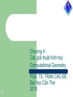
Figure 3.2 Depth-first-search of the largest connected component in the graph

CuuDuongThanCong.com

G

/>

Complexity of DFS

co

ng

.c
om

Property 3.4 Depth-firstsearch on a graph
represented by adjacency
lists requires time
proportional to V+ E.

cu

u

du
o

ng

th

an

So the result of DFS for the
graph in Figure 3.1a with
the adjacency lists in Figure
3.1c is
AFEGDCB
Note: the order of the vertices
in the adjacency lists has
influence on the order of
the DFS traversal.

Proof: We have to

initialize each element in
the array val (proportional
to O(V)), and check each
node in all the adjacency
lists which represent the
graph (proportional to
O(E)).
25

CuuDuongThanCong.com

/>