Tài liệu Ten Principles of Economics - Part 28 doc

CHAPTER 13 THE COSTS OF PRODUCTION 281
production process, the second or third worker might have higher marginal product
than the first because a team of workers can divide tasks and work more produc-
tively than a single worker. Such firms would first experience increasing marginal
product for a while before diminishing marginal product sets in.
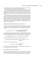
Table 13-3 shows the cost data for such a firm, called Big Bob’s Bagel Bin. These
data are graphed in Figure 13-6. Panel (a) shows how total cost (TC) depends on
the quantity produced, and panel (b) shows average total cost (ATC), average fixed
cost (AFC), average variable cost (AVC), and marginal cost (MC). In the range of
output from 0 to 4 bagels per hour, the firm experiences increasing marginal prod-
uct, and the marginal-cost curve falls. After 5 bagels per hour, the firm starts to ex-
perience diminishing marginal product, and the marginal-cost curve starts to rise.
This combination of increasing then diminishing marginal product also makes the
average-variable-cost curve U-shaped.
Despite these differences from our previous example, Big Bob’s cost curves
share the three properties that are most important to remember:
◆ Marginal cost eventually rises with the quantity of output.
◆ The average-total-cost curve is U-shaped.
◆ The marginal-cost curve crosses the average-total-cost curve at the minimum
of average total cost.
Table 13-3
Q
UANTITY AVERAGE AVERAGE AVERAGE
OF
BAGELS TOTAL FIXED VARIABLE FIXED VARIABLE TOTAL MARGINAL
(
PER HOUR)COST COST COST COST COST COST COST
0 $ 2.00 $2.00 $ 0.00 — — —
$1.00
1 3.00 2.00 1.00 $2.00 $1.00 $3.00
0.80

2 3.80 2.00 1.80 1.00 0.90 1.90
0.60
3 4.40 2.00 2.40 0.67 0.80 1.47
0.40
4 4.80 2.00 2.80 0.50 0.70 1.20
0.40
5 5.20 2.00 3.20 0.40 0.64 1.04
0.60
6 5.80 2.00 3.80 0.33 0.63 0.96
0.80
7 6.60 2.00 4.60 0.29 0.66 0.95
1.00
8 7.60 2.00 5.60 0.25 0.70 0.95
1.20
9 8.80 2.00 6.80 0.22 0.76 0.98
1.40
10 10.20 2.00 8.20 0.20 0.82 1.02
1.60
11 11.80 2.00 9.80 0.18 0.89 1.07
1.80
12 13.60 2.00 11.60 0.17 0.97 1.14
2.00
13 15.60 2.00 13.60 0.15 1.05 1.20
2.20
14 17.80 2.00 15.80 0.14 1.13 1.27
THE VARIOUS MEASURES OF COST: BIG BOB’S BAGEL BIN
282 PART FIVE FIRM BEHAVIOR AND THE ORGANIZATION OF INDUSTRY
0
(a) Total-Cost Curve
(b) Marginal- and Average-Cost Curves

Total
Cost
$18.00
17.00
16.00
15.00
14.00
13.00
12.00
11.00
10.00
9.00
8.00
7.00
6.00
5.00
4.00
3.00
Quantity of Output
(bagels per hour)
TC
Quantity of Output
(bagels per hour)
1432765981413121110
2.00
1.00
Costs
$3.00
2.75
2.50

2.25
2.00
1.75
1.50
1.25
1.00
0.75
0.50
0.25
0
1432765981413121110
MC
ATC
AVC
AFC
BIG BOB’S COST CURVES.Many
firms, like Big Bob’s Bagel Bin,
experience increasing marginal
product before diminishing
marginal product and, therefore,
have cost curves like those in this
figure. Panel (a) shows how total
cost (TC) depends on the quantity
produced. Panel (b) shows how
average total cost (ATC), average
fixed cost (AFC), average variable
cost (AVC), and marginal cost (MC)
depend on the quantity produced.
These curves are derived by
graphing the data from Table 13-3.

Notice that marginal cost and
average variable cost fall for a
while before starting to rise.
Figure 13-6
CHAPTER 13 THE COSTS OF PRODUCTION 283
QUICK QUIZ: Suppose Honda’s total cost of producing 4 cars is $225,000
and its total cost of producing 5 cars is $250,000. What is the average total cost
of producing 5 cars? What is the marginal cost of the fifth car? ◆ Draw the
marginal-cost curve and the average-total-cost curve for a typical firm, and
explain why these curves cross where they do.
COSTS IN THE SHORT RUN AND IN THE LONG RUN
We noted at the beginning of this chapter that a firm’s costs might depend on
the time horizon being examined. Let’s examine more precisely why this might be
the case.
THE RELATIONSHIP BETWEEN SHORT-RUN AND
LONG-RUN AVERAGE TOTAL COST
For many firms, the division of total costs between fixed and variable costs de-
pends on the time horizon. Consider, for instance, a car manufacturer, such as Ford
Motor Company. Over a period of only a few months, Ford cannot adjust the num-
ber or sizes of its car factories. The only way it can produce additional cars is to
hire more workers at the factories it already has. The cost of these factories is,
therefore, a fixed cost in the short run. By contrast, over a period of several years,
Ford can expand the size of its factories, build new factories, or close old ones.
Thus, the cost of its factories is a variable cost in the long run.
Because many decisions are fixed in the short run but variable in the long run,
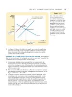
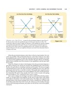
a firm’s long-run cost curves differ from its short-run cost curves. Figure 13-7
shows an example. The figure presents three short-run average-total-cost curves—
for a small, medium, and large factory. It also presents the long-run average-total-
cost curve. As the firm moves along the long-run curve, it is adjusting the size of
the factory to the quantity of production.

This graph shows how short-run and long-run costs are related. The long-run
average-total-cost curve is a much flatter U-shape than the short-run average-total-
cost curve. In addition, all the short-run curves lie on or above the long-run curve.
These properties arise because of the greater flexibility firms have in the long run.
In essence, in the long run, the firm gets to choose which short-run curve it wants
to use. But in the short run, it has to use whatever short-run curve it chose in
the past.
The figure shows an example of how a change in production alters costs over
different time horizons. When Ford wants to increase production from 1,000 to
1,200 cars per day, it has no choice in the short run but to hire more workers at its
existing medium-sized factory. Because of diminishing marginal product, average
total cost rises from $10,000 to $12,000 per car. In the long run, however, Ford can
expand both the size of the factory and its workforce, and average total cost re-
mains at $10,000.
How long does it take for a firm to get to the long run? The answer depends
on the firm. It can take a year or longer for a major manufacturing firm, such as a
284 PART FIVE FIRM BEHAVIOR AND THE ORGANIZATION OF INDUSTRY
car company, to build a larger factory. By contrast, a person running a lemonade
stand can go and buy a larger pitcher within an hour or less. There is, therefore, no
single answer about how long it takes a firm to adjust its production facilities.
ECONOMIES AND DISECONOMIES OF SCALE
The shape of the long-run average-total-cost curve conveys important information
about the technology for producing a good. When long-run average total cost de-
clines as output increases, there are said to be economies of scale. When long-run
average total cost rises as output increases, there are said to be diseconomies of
scale. When long-run average total cost does not vary with the level of output,
there are said to be constant returns to scale. In this example, Ford has economies
of scale at low levels of output, constant returns to scale at intermediate levels of
output, and diseconomies of scale at high levels of output.
What might cause economies or diseconomies of scale? Economies of scale

often arise because higher production levels allow specialization among workers,
which permits each worker to become better at his or her assigned tasks. For in-
stance, modern assembly-line production requires a large number of workers. If
Ford were producing only a small quantity of cars, it could not take advantage of
this approach and would have higher average total cost. Diseconomies of scale can
arise because of coordination problems that are inherent in any large organization.
The more cars Ford produces, the more stretched the management team becomes,
and the less effective the managers become at keeping costs down.
This analysis shows why long-run average-total-cost curves are often U-
shaped. At low levels of production, the firm benefits from increased size be-
cause it can take advantage of greater specialization. Coordination problems,
Quantity of
Cars per Day
0 1,2001,000
Average
Total
Cost
$12,000
10,000
Economies
of
scale
ATC
in short
run with
small factory
ATC
in short
run with
medium factory

ATC
in short
run with
large factory
ATC
in long run
Diseconomies
of
scale
Constant
returns to
scale
Figure 13-7
AVERAGE TOTAL COST IN THE
SHORT AND LONG RUNS.
Because fixed costs are variable in
the long run, the average-total-
cost curve in the short run differs
from the average-total-cost curve
in the long run.
economies of scale
the property whereby long-run
average total cost falls as the
quantity of output increases
diseconomies of scale
the property whereby long-run
average total cost rises as the
quantity of output increases
constant returns to scale
the property whereby long-run

average total cost stays the same as
the quantity of output changes
CHAPTER 13 THE COSTS OF PRODUCTION 285
meanwhile, are not yet acute. By contrast, at high levels of production, the benefits
of specialization have already been realized, and coordination problems become
more severe as the firm grows larger. Thus, long-run average total cost is falling at
low levels of production because of increasing specialization and rising at high
levels of production because of increasing coordination problems.
QUICK QUIZ: If Boeing produces 9 jets per month, its long-run total
cost is $9.0 million per month. If it produces 10 jets per month, its long-run
total cost is $9.5 million per month. Does Boeing exhibit economies or
diseconomies of scale?
CONCLUSION
The purpose of this chapter has been to develop some tools that we can use to study
how firms make production and pricing decisions. You should now understand
what economists mean by the term costs and how costs vary with the quantity of
output a firm produces. To refresh your memory, Table 13-4 summarizes some of
the definitions we have encountered.
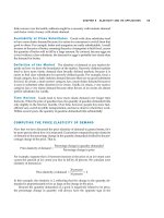
“Jack of all trades, master of
none.” This well-known adage
helps explain why firms some-
times experience economies of
scale. A person who tries to do
everything usually ends up doing
nothing very well. If a firm wants
its workers to be as productive
as they can be, it is often best
to give them a limited task that
they can master. But this is pos-
sible only if a firm employs a

large number of workers and
produces a large quantity of output.
In his celebrated book, An Inquiry into the Nature and
Causes of the Wealth of Nations, Adam Smith described an
example of this based on a visit he made to a pin factory.
Smith was impressed by the specialization among the work-
ers that he observed and the resulting economies of scale.
He wrote,
“One man draws out the wire, another straightens it, a
third cuts it, a fourth points it, a fifth grinds it at the top
for receiving the head; to make the head requires two or
three distinct operations; to put it on is a peculiar
business; to whiten it is another; it is even a trade by
itself to put them into paper.”
Smith reported that because of this specialization, the pin
factory produced thousands of pins per worker every day.
He conjectured that if the workers had chosen to work sep-
arately, rather than as a team of specialists, “they certainly
could not each of them make twenty, perhaps not one pin a
day.” In other words, because of specialization, a large pin
factory could achieve higher output per worker and lower av-
erage cost per pin than a small pin factory.
The specialization that Smith observed in the pin fac-
tory is prevalent in the modern economy. If you want to build
a house, for instance, you could try to do all the work your-
self. But most people turn to a builder, who in turn hires
carpenters, plumbers, electricians, painters, and many other
types of worker. These workers specialize in particular jobs,
and this allows them to become better at their jobs than if
they were generalists. Indeed, the use of specialization to

achieve economies of scale is one reason modern societies
are as prosperous as they are.
FYI
Lessons from a
Pin Factory
286 PART FIVE FIRM BEHAVIOR AND THE ORGANIZATION OF INDUSTRY
By themselves, of course, a firm’s cost curves do not tell us what decisions the
firm will make. But they are an important component of that decision, as we will
begin to see in the next chapter.
Table 13-4
THE MANY TYPES OF COST:
AS
UMMARY
M
ATHEMATICAL
TERM DEFINITION DESCRIPTION
Explicit costs Costs that require an outlay of —
money by the firm
Implicit costs Costs that do not require an outlay —
of money by the firm
Fixed costs Costs that do not vary with the FC
quantity of output produced
Variable costs Costs that do vary with the VC
quantity of output produced
Total cost The market value of all the inputs TC ϭ FC ϩ VC
that a firm uses in production
Average fixed cost Fixed costs divided by the quantity AFC ϭ FC/Q
of output
Average variable cost Variable costs divided by the AVC ϭ VC/Q
quantity of output

Average total cost Total cost divided by the quantity ATC ϭ TC/Q
of output
Marginal cost The increase in total cost that arises MC ϭ⌬TC/⌬Q
from an extra unit of production
◆ The goal of firms is to maximize profit, which equals
total revenue minus total cost.
◆ When analyzing a firm’s behavior, it is important to
include all the opportunity costs of production. Some of
the opportunity costs, such as the wages a firm pays its
workers, are explicit. Other opportunity costs, such as
the wages the firm owner gives up by working in the
firm rather than taking another job, are implicit.
◆ A firm’s costs reflect its production process. A typical
firm’s production function gets flatter as the quantity
of an input increases, displaying the property of
diminishing marginal product. As a result, a firm’s
total-cost curve gets steeper as the quantity produced
rises.
◆ A firm’s total costs can be divided between fixed costs
and variable costs. Fixed costs are costs that do not
change when the firm alters the quantity of output
produced. Variable costs are costs that do change when
the firm alters the quantity of output produced.
◆ From a firm’s total cost, two related measures of cost are
derived. Average total cost is total cost divided by the
quantity of output. Marginal cost is the amount by
which total cost would rise if output were increased by
1 unit.
◆ When analyzing firm behavior, it is often useful to
graph average total cost and marginal cost. For a typical

firm, marginal cost rises with the quantity of output.
Average total cost first falls as output increases and then
Summary
CHAPTER 13 THE COSTS OF PRODUCTION 287
rises as output increases further. The marginal-cost
curve always crosses the average-total-cost curve at the
minimum of average total cost.
◆ A firm’s costs often depend on the time horizon being
considered. In particular, many costs are fixed in the
short run but variable in the long run. As a result, when
the firm changes its level of production, average total
cost may rise more in the short run than in the long run.
total revenue, p. 270
total cost, p. 270
profit, p. 270
explicit costs, p. 271
implicit costs, p. 271
economic profit, p. 272
accounting profit, p. 272
production function, p. 273
marginal product, p. 273
diminishing marginal product, p. 273
fixed costs, p. 277
variable costs, p. 277
average total cost, p. 278
average fixed cost, p. 278
average variable cost, p. 278
marginal cost, p. 278
efficient scale, p. 280
economies of scale, p. 284

diseconomies of scale, p. 284
constant returns to scale, p. 284
Key Concepts
1. What is the relationship between a firm’s total revenue,
profit, and total cost?
2. Give an example of an opportunity cost that an
accountant might not count as a cost. Why would the
accountant ignore this cost?
3. What is marginal product, and what does it mean if it is
diminishing?
4. Draw a production function that exhibits diminishing
marginal product of labor. Draw the associated total-
cost curve. (In both cases, be sure to label the axes.)
Explain the shapes of the two curves you have drawn.
5. Define total cost, average total cost, and marginal cost.
How are they related?
6. Draw the marginal-cost and average-total-cost curves
for a typical firm. Explain why the curves have the
shapes that they do and why they cross where they do.
7. How and why does a firm’s average-total-cost curve
differ in the short run and in the long run?
8. Define economies of scale and explain why they might
arise. Define diseconomies of scale and explain why they
might arise.
Questions for Review
1. This chapter discusses many types of costs: opportunity
cost, total cost, fixed cost, variable cost, average total
cost, and marginal cost. Fill in the type of cost that best
completes the phrases below:
a. The true cost of taking some action is its _______.

b. _______ is falling when marginal cost is below it,
and rising when marginal cost is above it.
c. A cost that does not depend on the quantity
produced is a _______.
d. In the ice-cream industry in the short run, _______
includes the cost of cream and sugar, but not the
cost of the factory.
e. Profits equal total revenue less _______.
f. The cost of producing an extra unit of output is
_______.
2. Your aunt is thinking about opening a hardware store.
She estimates that it would cost $500,000 per year to rent
the location and buy the stock. In addition, she would
have to quit her $50,000 per year job as an accountant.
a. Define opportunity cost.
b. What is your aunt’s opportunity cost of running a
hardware store for a year? If your aunt thought she
could sell $510,000 worth of merchandise in a year,
should she open the store? Explain.
Problems and Applications
288 PART FIVE FIRM BEHAVIOR AND THE ORGANIZATION OF INDUSTRY
3. Suppose that your college charges you separately for
tuition and for room and board.
a. What is a cost of attending college that is not an
opportunity cost?
b. What is an explicit opportunity cost of attending
college?
c. What is an implicit opportunity cost of attending
college?
4. A commercial fisherman notices the following

relationship between hours spent fishing and the
quantity of fish caught:
HOURS QUANTITY OF FISH (IN POUNDS)
00
110
218
324
428
530
a. What is the marginal product of each hour spent
fishing?
b. Use these data to graph the fisherman’s production
function. Explain its shape.
c. The fisherman has a fixed cost of $10 (his pole). The
opportunity cost of his time is $5 per hour. Graph
the fisherman’s total-cost curve. Explain its shape.
5. Nimbus, Inc., makes brooms and then sells them door-
to-door. Here is the relationship between the number of
workers and Nimbus’s output in a given day:
AVERAGE
M
ARGINAL TOTAL TOTAL MARGINAL
WORKERS OUTPUT PRODUCT COST COST COST
0 0 _______ _______
_______ ______
1 20 _______ _______
_______ _______
2 50 _______ _______
_______ _______
3 90 _______ _______

_______ _______
4 120 _______ _______
_______ _______
5 140 _______ _______
_______ _______
6 150 _______ _______
_______ _______
7 155 _______ _______
a. Fill in the column of marginal products. What
pattern do you see? How might you explain it?
b. A worker costs $100 a day, and the firm has fixed
costs of $200. Use this information to fill in the
column for total cost.
c. Fill in the column for average total cost. (Recall that
ATC = TC/Q.) What pattern do you see?
d. Now fill in the column for marginal cost. (Recall
that MC = ⌬TC/⌬Q.) What pattern do you see?
e. Compare the column for marginal product and the
column for marginal cost. Explain the relationship.
f. Compare the column for average total cost and the
column for marginal cost. Explain the relationship.
6. Suppose that you and your roommate have started a
bagel delivery service on campus. List some of your
fixed costs and describe why they are fixed. List some of
your variable costs and describe why they are variable.
7. Consider the following cost information for a pizzeria:
Q (DOZENS)TOTAL COST VARIABLE COST
0 $300 $ 0
1 350 50
2 390 90

3 420 120
4 450 150
5 490 190
6 540 240
a. What is the pizzeria’s fixed cost?
b. Construct a table in which you calculate the
marginal cost per dozen pizzas using the
information on total cost. Also calculate the
marginal cost per dozen pizzas using the
information on variable cost. What is the
relationship between these sets of numbers?
Comment.
8. You are thinking about setting up a lemonade stand.
The stand itself costs $200. The ingredients for each cup
of lemonade cost $0.50.
a. What is your fixed cost of doing business? What is
your variable cost per cup?
b. Construct a table showing your total cost, average
total cost, and marginal cost for output levels
varying from zero to 10 gallons. (Hint: There are 16
cups in a gallon.) Draw the three cost curves.
9. Your cousin Vinnie owns a painting company with fixed
costs of $200 and the following schedule for variable
costs:
CHAPTER 13 THE COSTS OF PRODUCTION 289
Q
UANTITY OF HOUSES
P
AINTED PER MONTH
1234 5 6 7

Variable costs $10 $20 $40 $80 $160 $320 $640
Calculate average fixed cost, average variable cost, and
average total cost for each quantity. What is the efficient
scale of the painting company?
10. Healthy Harry’s Juice Bar has the following cost
schedules:
Q (VAT S )VARIABLE COST TOTAL COST
0$0 $ 30
110 40
225 55
345 75
4 70 100
5 100 130
6 135 165
a. Calculate average variable cost, average total cost,
and marginal cost for each quantity.
b. Graph all three curves. What is the relationship
between the marginal-cost curve and the average-
total-cost curve? Between the marginal-cost curve
and the average-variable-cost curve? Explain.
11. Consider the following table of long-run total cost for
three different firms:
QUANTITY
123 4 5 6 7
Firm A $60 $70 $80 $90 $100 $110 $120
Firm B 11 24 39 56 75 96 119
Firm C 21 34 49 66 85 106 129
Does each of these firms experience economies of scale
or diseconomies of scale?