Tài liệu Ten Principles of Economics - Part 32 doc

CHAPTER 15 MONOPOLY 321
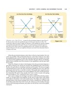
perfect substitutes (the products of all the other firms in its market), the demand
curve that any one firm faces is perfectly elastic.
By contrast, because a monopoly is the sole producer in its market, its de-
mand curve is the market demand curve. Thus, the monopolist’s demand curve
slopes downward for all the usual reasons, as in panel (b) of Figure 15-2. If the mo-
nopolist raises the price of its good, consumers buy less of it. Looked at another way,
if the monopolist reduces the quantity of output it sells, the price of its output
increases.
The market demand curve provides a constraint on a monopoly’s ability to
profit from its market power. A monopolist would prefer, if it were possible, to
charge a high price and sell a large quantity at that high price. The market demand
curve makes that outcome impossible. In particular, the market demand curve de-
scribes the combinations of price and quantity that are available to a monopoly
firm. By adjusting the quantity produced (or, equivalently, the price charged), the
monopolist can choose any point on the demand curve, but it cannot choose a
point off the demand curve.
What point on the demand curve will the monopolist choose? As with com-
petitive firms, we assume that the monopolist’s goal is to maximize profit. Because
the firm’s profit is total revenue minus total costs, our next task in explaining mo-
nopoly behavior is to examine a monopolist’s revenue.
A MONOPOLY’S REVENUE
Consider a town with a single producer of water. Table 15-1 shows how the mo-
nopoly’s revenue might depend on the amount of water produced.
The first two columns show the monopolist’s demand schedule. If the mo-
nopolist produces 1 gallon of water, it can sell that gallon for $10. If it produces
Table 15-1
QUANTITY
OF WATER PRICE TOTAL REVENUE AVERAGE REVENUE MARGINAL REVENUE
(Q)(P)(TR ؍ P ؋ Q)(AR ؍ TR/Q)(MR ؍⌬TR/⌬Q)
0 gallons $11 $ 0 —

$10
1 10 10 $10
8
2918 9
6
3824 8
4
4728 7
2
5630 6
0
6530 5
Ϫ2
7428 4
Ϫ4
8324 3
AMONOPOLY’S TOTAL, AVERAGE, AND MARGINAL REVENUE
322 PART FIVE FIRM BEHAVIOR AND THE ORGANIZATION OF INDUSTRY
2 gallons, it must lower the price to $9 in order to sell both gallons. And if it
produces 3 gallons, it must lower the price to $8. And so on. If you graphed these
two columns of numbers, you would get a typical downward-sloping demand
curve.
The third column of the table presents the monopolist’s total revenue. It equals
the quantity sold (from the first column) times the price (from the second column).
The fourth column computes the firm’s average revenue, the amount of revenue the
firm receives per unit sold. We compute average revenue by taking the number
for total revenue in the third column and dividing it by the quantity of output
in the first column. As we discussed in Chapter 14, average revenue always
equals the price of the good. This is true for monopolists as well as for competitive
firms.

The last column of Table 15-1 computes the firm’s marginal revenue, the amount
of revenue that the firm receives for each additional unit of output. We compute
marginal revenue by taking the change in total revenue when output increases by
1 unit. For example, when the firm is producing 3 gallons of water, it receives total
revenue of $24. Raising production to 4 gallons increases total revenue to $28.
Thus, marginal revenue is $28 minus $24, or $4.
Table 15-1 shows a result that is important for understanding monopoly be-
havior: A monopolist’s marginal revenue is always less than the price of its good. For ex-
ample, if the firm raises production of water from 3 to 4 gallons, it will increase
total revenue by only $4, even though it will be able to sell each gallon for $7. For
a monopoly, marginal revenue is lower than price because a monopoly faces a
downward-sloping demand curve. To increase the amount sold, a monopoly firm
must lower the price of its good. Hence, to sell the fourth gallon of water, the mo-
nopolist must get less revenue for each of the first three gallons.
Marginal revenue is very different for monopolies from what it is for compet-
itive firms. When a monopoly increases the amount it sells, it has two effects on to-
tal revenue (P ϫ Q):
◆ The output effect: More output is sold, so Q is higher.
◆ The price effect: The price falls, so P is lower.
Because a competitive firm can sell all it wants at the market price, there is no price
effect. When it increases production by 1 unit, it receives the market price for that
unit, and it does not receive any less for the amount it was already selling. That is,
because the competitive firm is a price taker, its marginal revenue equals the price
of its good. By contrast, when a monopoly increases production by 1 unit, it must
reduce the price it charges for every unit it sells, and this cut in price reduces rev-
enue on the units it was already selling. As a result, a monopoly’s marginal rev-
enue is less than its price.
Figure 15-3 graphs the demand curve and the marginal-revenue curve for a
monopoly firm. (Because the firm’s price equals its average revenue, the demand
curve is also the average-revenue curve.) These two curves always start at the

same point on the vertical axis because the marginal revenue of the first unit sold
equals the price of the good. But, for the reason we just discussed, the monopolist’s
marginal revenue is less than the price of the good. Thus, a monopoly’s marginal-
revenue curve lies below its demand curve.
You can see in the figure (as well as in Table 15-1) that marginal revenue can
even become negative. Marginal revenue is negative when the price effect on
CHAPTER 15 MONOPOLY 323
revenue is greater than the output effect. In this case, when the firm produces an
extra unit of output, the price falls by enough to cause the firm’s total revenue to
decline, even though the firm is selling more units.
PROFIT MAXIMIZATION
Now that we have considered the revenue of a monopoly firm, we are ready to
examine how such a firm maximizes profit. Recall from Chapter 1 that one of
the Ten Principles of Economics is that rational people think at the margin. This
lesson is as true for monopolists as it is for competitive firms. Here we apply the
logic of marginal analysis to the monopolist’s problem of deciding how much to
produce.
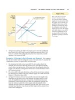
Figure 15-4 graphs the demand curve, the marginal-revenue curve, and the
cost curves for a monopoly firm. All these curves should seem familiar: The de-
mand and marginal-revenue curves are like those in Figure 15-3, and the cost
curves are like those we introduced in Chapter 13 and used to analyze competitive
firms in Chapter 14. These curves contain all the information we need to determine
the level of output that a profit-maximizing monopolist will choose.
Suppose, first, that the firm is producing at a low level of output, such as Q
1
.
In this case, marginal cost is less than marginal revenue. If the firm increased pro-
duction by 1 unit, the additional revenue would exceed the additional costs, and
profit would rise. Thus, when marginal cost is less than marginal revenue, the firm
can increase profit by producing more units.

Quantity of Water
Price
$11
10
9
8
7
6
5
4
3
2
1
0
Ϫ1
Ϫ2
Ϫ3
Ϫ4
Demand
(average
revenue)
Marginal
revenue
12345 678
Figure 15-3
DEMAND AND MARGINAL-
R
EVENUE CURVES FOR A
MONOPOLY. The demand
curve shows how the quantity

affects the price of the good. The
marginal-revenue curve shows
how the firm’s revenue changes
when the quantity increases by
1 unit. Because the price on all
units sold must fall if the
monopoly increases production,
marginal revenue is always less
than the price.
324 PART FIVE FIRM BEHAVIOR AND THE ORGANIZATION OF INDUSTRY
A similar argument applies at high levels of output, such as Q
2
. In this case,
marginal cost is greater than marginal revenue. If the firm reduced production by
1 unit, the costs saved would exceed the revenue lost. Thus, if marginal cost is
greater than marginal revenue, the firm can raise profit by reducing production.
In the end, the firm adjusts its level of production until the quantity reaches
Q
MAX
, at which marginal revenue equals marginal cost. Thus, the monopolist’s profit-
maximizing quantity of output is determined by the intersection of the marginal-revenue
curve and the marginal-cost curve. In Figure 15-4, this intersection occurs at point A.
You might recall from Chapter 14 that competitive firms also choose the quan-
tity of output at which marginal revenue equals marginal cost. In following this
rule for profit maximization, competitive firms and monopolies are alike. But there
is also an important difference between these types of firm: The marginal revenue
of a competitive firm equals its price, whereas the marginal revenue of a monop-
oly is less than its price. That is,
For a competitive firm: P ϭ MR ϭ MC.
For a monopoly firm: P > MR ϭ MC.

The equality of marginal revenue and marginal cost at the profit-maximizing
quantity is the same for both types of firm. What differs is the relationship of the
price to marginal revenue and marginal cost.
How does the monopoly find the profit-maximizing price for its product? The
demand curve answers this question, for the demand curve relates the amount
that customers are willing to pay to the quantity sold. Thus, after the monopoly
firm chooses the quantity of output that equates marginal revenue and marginal
Monopoly
price
Quantity
Q
1
Q
2
Q
MAX
0
Costs and
Revenue
Demand
Average total cost
Marginal revenue
Marginal
cost
B
1. The intersection of the
marginal-revenue curve
and the marginal-cost
curve determines the
profit-maximizing

quantity . . .
A
2. . . . and then the demand
curve shows the price
consistent with this quantity.
Figure 15-4
PROFIT MAXIMIZATION FOR A
MONOPOLY. A monopoly
maximizes profit by choosing the
quantity at which marginal
revenue equals marginal cost
(point A). It then uses the
demand curve to find the price
that will induce consumers to
buy that quantity (point B).
CHAPTER 15 MONOPOLY 325
cost, it uses the demand curve to find the price consistent with that quantity. In
Figure 15-4, the profit-maximizing price is found at point B.
We can now see a key difference between markets with competitive firms and
markets with a monopoly firm: In competitive markets, price equals marginal cost. In
monopolized markets, price exceeds marginal cost. As we will see in a moment, this
finding is crucial to understanding the social cost of monopoly.
A MONOPOLY’S PROFIT
How much profit does the monopoly make? To see the monopoly’s profit, recall
that profit equals total revenue (TR) minus total costs (TC):
Profit ϭ TR Ϫ TC.
We can rewrite this as
Profit ϭ (TR/Q Ϫ TC/Q) ϫ Q.
TR/Q is average revenue, which equals the price P, and TC/Q is average total cost
ATC. Therefore,

Profit ϭ (P Ϫ ATC) ϫ Q.
This equation for profit (which is the same as the profit equation for competitive
firms) allows us to measure the monopolist’s profit in our graph.
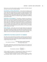
Consider the shaded box in Figure 15-5. The height of the box (the segment
BC) is price minus average total cost, P – ATC, which is the profit on the typical
unit sold. The width of the box (the segment DC) is the quantity sold Q
MAX
. There-
fore, the area of this box is the monopoly firm’s total profit.
You may have noticed that we
have analyzed the price in a
monopoly market using the
market demand curve and the
firm’s cost curves. We have not
made any mention of the mar-
ket supply curve. By contrast,
when we analyzed prices in
competitive markets beginning
in Chapter 4, the two most im-
portant words were always sup-
ply and demand.
What happened to the sup-
ply curve? Although monopoly firms make decisions about
what quantity to supply (in the way described in this chapter),
a monopoly does not have a supply curve. A supply curve
tells us the quantity that firms choose to supply at any given
price. This concept makes sense when we are analyzing com-
petitive firms, which are price takers. But a monopoly firm is
a price maker, not a price taker. It is not meaningful to ask
what such a firm would produce at any price because the

firm sets the price at the same time it chooses the quantity
to supply.
Indeed, the monopolist’s decision about how much to
supply is impossible to separate from the demand curve it
faces. The shape of the demand curve determines the
shape of the marginal-revenue curve, which in turn deter-
mines the monopolist’s profit-maximizing quantity. In a com-
petitive market, supply decisions can be analyzed without
knowing the demand curve, but that is not true in a monop-
oly market. Therefore, we never talk about a monopoly’s
supply curve.
FYI
Why a
Monopoly Does
Not Have a
Supply Curve
326 PART FIVE FIRM BEHAVIOR AND THE ORGANIZATION OF INDUSTRY
CASE STUDY MONOPOLY DRUGS VERSUS GENERIC DRUGS
According to our analysis, prices are determined quite differently in monopo-
lized markets from the way they are in competitive markets. A natural place to
test this theory is the market for pharmaceutical drugs because this market
takes on both market structures. When a firm discovers a new drug, patent laws
give the firm a monopoly on the sale of that drug. But eventually the firm’s
patent runs out, and any company can make and sell the drug. At that time, the
market switches from being monopolistic to being competitive.
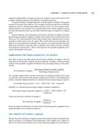
What should happen to the price of a drug when the patent runs out?
Figure 15-6 shows the market for a typical drug. In this figure, the marginal cost
of producing the drug is constant. (This is approximately true for many drugs.)
During the life of the patent, the monopoly firm maximizes profit by produc-
ing the quantity at which marginal revenue equals marginal cost and charging

a price well above marginal cost. But when the patent runs out, the profit
from making the drug should encourage new firms to enter the market. As the
market becomes more competitive, the price should fall to equal marginal cost.
Experience is, in fact, consistent with our theory. When the patent on a drug
expires, other companies quickly enter and begin selling so-called generic
products that are chemically identical to the former monopolist’s brand-name
product. And just as our analysis predicts, the price of the competitively pro-
duced generic drug is well below the price that the monopolist was charging.
The expiration of a patent, however, does not cause the monopolist to lose
all its market power. Some consumers remain loyal to the brand-name drug,
perhaps out of fear that the new generic drugs are not actually the same as the
drug they have been using for years. As a result, the former monopolist can
continue to charge a price at least somewhat above the price charged by its
new competitors.
Monopoly
price
Average
total
cost
Quantity
Q
MAX
0
Costs and
Revenue
Demand
Marginal cost
Marginal revenue
B
C

E
D
Monopoly
profit
Average total cost
Figure 15-5
THE MONOPOLIST’S PROFIT.
The area of the box BCDE equals
the profit of the monopoly firm.
The height of the box (BC) is
price minus average total cost,
which equals profit per unit sold.
The width of the box (DC) is the
number of units sold.
CHAPTER 15 MONOPOLY 327
QUICK QUIZ: Explain how a monopolist chooses the quantity of output to
produce and the price to charge.
THE WELFARE COST OF MONOPOLY
Is monopoly a good way to organize a market? We have seen that a monopoly, in
contrast to a competitive firm, charges a price above marginal cost. From the stand-
point of consumers, this high price makes monopoly undesirable. At the same time,
however, the monopoly is earning profit from charging this high price. From the
standpoint of the owners of the firm, the high price makes monopoly very desirable.
Is it possible that the benefits to the firm’s owners exceed the costs imposed on con-
sumers, making monopoly desirable from the standpoint of society as a whole?
We can answer this question using the type of analysis we first saw in Chapter
7. As in that chapter, we use total surplus as our measure of economic well-being.
Recall that total surplus is the sum of consumer surplus and producer surplus.
Consumer surplus is consumers’ willingness to pay for a good minus the amount
they actually pay for it. Producer surplus is the amount producers receive for a

good minus their costs of producing it. In this case, there is a single producer: the
monopolist.
You might already be able to guess the result of this analysis. In Chapter 7 we
concluded that the equilibrium of supply and demand in a competitive market is
not only a natural outcome but a desirable one. In particular, the invisible hand of
the market leads to an allocation of resources that makes total surplus as large as
it can be. Because a monopoly leads to an allocation of resources different from
that in a competitive market, the outcome must, in some way, fail to maximize to-
tal economic well-being.
Price
during
patent life
Price after
patent
expires
QuantityMonopoly
quantity
Competitive
quantity
0
Costs and
Revenue
Demand
Marginal
cost
Marginal
revenue
Figure 15-6
THE MARKET FOR DRUGS.
When a patent gives a firm a

monopoly over the sale of a
drug, the firm charges the
monopoly price, which is well
above the marginal cost of
making the drug. When the
patent on a drug runs out, new
firms enter the market, making
it more competitive. As a result,
the price falls from the monopoly
price to marginal cost.
328 PART FIVE FIRM BEHAVIOR AND THE ORGANIZATION OF INDUSTRY
THE DEADWEIGHT LOSS
We begin by considering what the monopoly firm would do if it were run by a
benevolent social planner. The social planner cares not only about the profit
earned by the firm’s owners but also about the benefits received by the firm’s con-
sumers. The planner tries to maximize total surplus, which equals producer sur-
plus (profit) plus consumer surplus. Keep in mind that total surplus equals the
value of the good to consumers minus the costs of making the good incurred by
the monopoly producer.
Figure 15-7 analyzes what level of output a benevolent social planner would
choose. The demand curve reflects the value of the good to consumers, as mea-
sured by their willingness to pay for it. The marginal-cost curve reflects the costs
of the monopolist. Thus, the socially efficient quantity is found where the demand curve
and the marginal-cost curve intersect. Below this quantity, the value to consumers ex-
ceeds the marginal cost of providing the good, so increasing output would raise to-
tal surplus. Above this quantity, the marginal cost exceeds the value to consumers,
so decreasing output would raise total surplus.
If the social planner were running the monopoly, the firm could achieve this ef-
ficient outcome by charging the price found at the intersection of the demand and
marginal-cost curves. Thus, like a competitive firm and unlike a profit-maximizing

monopoly, a social planner would charge a price equal to marginal cost. Because
this price would give consumers an accurate signal about the cost of producing the
good, consumers would buy the efficient quantity.
We can evaluate the welfare effects of monopoly by comparing the level of
output that the monopolist chooses to the level of output that a social planner
Quantity0
Price
Demand
(value to buyers)
Efficient
quantity
Marginal cost
Value to buyers
is greater than
cost to seller.
Value to buyers
is less than
cost to seller.
Cost
to
monopolist
Cost
to
monopolist
Value
to
buyers
Value
to
buyers

Figure 15-7
THE EFFICIENT LEVEL OF
OUTPUT. A benevolent social
planner who wanted to maximize
total surplus in the market would
choose the level of output where
the demand curve and marginal-
cost curve intersect. Below this
level, the value of the good to the
marginal buyer (as reflected in
the demand curve) exceeds the
marginal cost of making the
good. Above this level, the value
to the marginal buyer is less than
marginal cost.
CHAPTER 15 MONOPOLY 329
would choose. As we have seen, the monopolist chooses to produce and sell the
quantity of output at which the marginal-revenue and marginal-cost curves in-
tersect; the social planner would choose the quantity at which the demand and
marginal-cost curves intersect. Figure 15-8 shows the comparison. The monopolist
produces less than the socially efficient quantity of output.
We can also view the inefficiency of monopoly in terms of the monopolist’s
price. Because the market demand curve describes a negative relationship between
the price and quantity of the good, a quantity that is inefficiently low is equivalent
to a price that is inefficiently high. When a monopolist charges a price above mar-
ginal cost, some potential consumers value the good at more than its marginal cost
but less than the monopolist’s price. These consumers do not end up buying the
good. Because the value these consumers place on the good is greater than the cost
of providing it to them, this result is inefficient. Thus, monopoly pricing prevents
some mutually beneficial trades from taking place.

Just as we measured the inefficiency of taxes with the deadweight-loss triangle
in Chapter 8, we can similarly measure the inefficiency of monopoly. Figure 15-8
shows the deadweight loss. Recall that the demand curve reflects the value to con-
sumers and the marginal-cost curve reflects the costs to the monopoly producer.
Thus, the area of the deadweight-loss triangle between the demand curve and the
marginal-cost curve equals the total surplus lost because of monopoly pricing.
The deadweight loss caused by monopoly is similar to the deadweight loss
caused by a tax. Indeed, a monopolist is like a private tax collector. As we saw in
Chapter 8, a tax on a good places a wedge between consumers’ willingness to pay
(as reflected in the demand curve) and producers’ costs (as reflected in the supply
curve). Because a monopoly exerts its market power by charging a price above
marginal cost, it places a similar wedge. In both cases, the wedge causes the quan-
tity sold to fall short of the social optimum. The difference between the two cases
is that the government gets the revenue from a tax, whereas a private firm gets the
monopoly profit.
Quantity0
Price
Efficient
quantity
Monopoly
price
Monopoly
quantity
Deadweight
loss
Demand
Marginal
revenue
Marginal cost
Figure 15-8

THE INEFFICIENCY OF
MONOPOLY. Because a
monopoly charges a price above
marginal cost, not all consumers
who value the good at more than
its cost buy it. Thus, the quantity
produced and sold by a
monopoly is below the socially
efficient level. The deadweight
loss is represented by the area of
the triangle between the demand
curve (which reflects the value of
the good to consumers) and the
marginal-cost curve (which
reflects the costs of the monopoly
producer).
330 PART FIVE FIRM BEHAVIOR AND THE ORGANIZATION OF INDUSTRY
THE MONOPOLY’S PROFIT: A SOCIAL COST?
It is tempting to decry monopolies for “profiteering” at the expense of the public.
And, indeed, a monopoly firm does earn a higher profit by virtue of its market
power. According to the economic analysis of monopoly, however, the firm’s profit
is not in itself necessarily a problem for society.
Welfare in a monopolized market, like all markets, includes the welfare of both
consumers and producers. Whenever a consumer pays an extra dollar to a producer
because of a monopoly price, the consumer is worse off by a dollar, and the producer
is better off by the same amount. This transfer from the consumers of the good to the
owners of the monopoly does not affect the market’s total surplus—the sum of con-
sumer and producer surplus. In other words, the monopoly profit itself does not
represent a shrinkage in the size of the economic pie; it merely represents a bigger
slice for producers and a smaller slice for consumers. Unless consumers are for some

reason more deserving than producers—a judgment that goes beyond the realm of
economic efficiency—the monopoly profit is not a social problem.
The problem in a monopolized market arises because the firm produces and
sells a quantity of output below the level that maximizes total surplus. The dead-
weight loss measures how much the economic pie shrinks as a result. This ineffi-
ciency is connected to the monopoly’s high price: Consumers buy fewer units
when the firm raises its price above marginal cost. But keep in mind that the profit
earned on the units that continue to be sold is not the problem. The problem stems
from the inefficiently low quantity of output. Put differently, if the high monopoly
price did not discourage some consumers from buying the good, it would raise
producer surplus by exactly the amount it reduced consumer surplus, leaving to-
tal surplus the same as could be achieved by a benevolent social planner.
There is, however, a possible exception to this conclusion. Suppose that a mo-
nopoly firm has to incur additional costs to maintain its monopoly position. For
example, a firm with a government-created monopoly might need to hire lobbyists
to convince lawmakers to continue its monopoly. In this case, the monopoly may
use up some of its monopoly profits paying for these additional costs. If so, the so-
cial loss from monopoly includes both these costs and the deadweight loss result-
ing from a price above marginal cost.
QUICK QUIZ: How does a monopolist’s quantity of output compare to the
quantity of output that maximizes total surplus?
PUBLIC POLICY TOWARD MONOPOLIES
We have seen that monopolies, in contrast to competitive markets, fail to allocate
resources efficiently. Monopolies produce less than the socially desirable quantity
of output and, as a result, charge prices above marginal cost. Policymakers in the
government can respond to the problem of monopoly in one of four ways:
◆ By trying to make monopolized industries more competitive
◆ By regulating the behavior of the monopolies