Tài liệu Ten Principles of Economics - Part 75 pdf

CHAPTER 33 THE SHORT-RUN TRADEOFF BETWEEN INFLATION AND UNEMPLOYMENT 765
In panel (b) of the figure, we can see what these two possible outcomes mean
for unemployment and inflation. Because firms need more workers when they
produce a greater output of goods and services, unemployment is lower in out-
come B than in outcome A. In this example, when output rises from 7,500 to 8,000,
unemployment falls from 7 percent to 4 percent. Moreover, because the price level
is higher at outcome B than at outcome A, the inflation rate (the percentage change
in the price level from the previous year) is also higher. In particular, since the
price level was 100 in year 2000, outcome A has an inflation rate of 2 percent, and
outcome B has an inflation rate of 6 percent. Thus, we can compare the two possi-
ble outcomes for the economy either in terms of output and the price level (using
the model of aggregate demand and aggregate supply) or in terms of unemploy-
ment and inflation (using the Phillips curve).
As we saw in the preceding chapter, monetary and fiscal policy can shift
the aggregate-demand curve. Therefore, monetary and fiscal policy can move the
economy along the Phillips curve. Increases in the money supply, increases in
government spending, or cuts in taxes expand aggregate demand and move the
economy to a point on the Phillips curve with lower unemployment and higher
inflation. Decreases in the money supply, cuts in government spending, or in-
creases in taxes contract aggregate demand and move the economy to a point
on the Phillips curve with lower inflation and higher unemployment. In this sense,
the Phillips curve offers policymakers a menu of combinations of inflation and
unemployment.
QUICK QUIZ: Draw the Phillips curve. Use the model of aggregate
demand and aggregate supply to show how policy can move the economy
from a point on this curve with high inflation to a point with low inflation.
SHIFTS IN THE PHILLIPS CURVE:
THE ROLE OF EXPECTATIONS
The Phillips curve seems to offer policymakers a menu of possible inflation-
unemployment outcomes. But does this menu remain stable over time? Is the
Phillips curve a relationship on which policymakers can rely? Economists took up

these questions in the late 1960s, shortly after Samuelson and Solow had intro-
duced the Phillips curve into the macroeconomic policy debate.
THE LONG-RUN PHILLIPS CURVE
In 1968 economist Milton Friedman published a paper in the American Economic
Review, based on an address he had recently given as president of the American
Economic Association. The paper, titled “The Role of Monetary Policy,” contained
sections on “What Monetary Policy Can Do” and “What Monetary Policy Cannot
Do.” Friedman argued that one thing monetary policy cannot do, other than for
only a short time, is pick a combination of inflation and unemployment on the
Phillips curve. At about the same time, another economist, Edmund Phelps, also
766 PART TWELVE SHORT-RUN ECONOMIC FLUCTUATIONS
published a paper denying the existence of a long-run tradeoff between inflation
and unemployment.
Friedman and Phelps based their conclusions on classical principles of macro-
economics, which we discussed in Chapters 24 through 30. Recall that classical
theory points to growth in the money supply as the primary determinant of infla-
tion. But classical theory also states that monetary growth does not have real ef-
fects—it merely alters all prices and nominal incomes proportionately. In
particular, monetary growth does not influence those factors that determine the
economy’s unemployment rate, such as the market power of unions, the role of ef-
ficiency wages, or the process of job search. Friedman and Phelps concluded that
there is no reason to think the rate of inflation would, in the long run, be related to
the rate of unemployment.
Here, in his own words, is Friedman’s view about what the Fed can hope to
accomplish in the long run:
The monetary authority controls nominal quantities—directly, the quantity of its
own liabilities [currency plus bank reserves]. In principle, it can use this control
to peg a nominal quantity—an exchange rate, the price level, the nominal level of
national income, the quantity of money by one definition or another—or to peg
the change in a nominal quantity—the rate of inflation or deflation, the rate of

ACCORDING TO THE PHILLIPS CURVE, WHEN
unemployment falls to low levels,
wages and prices start to rise more
quickly. The following article illustrates
this link between labor-market condi-
tions and inflation.
Tighter Labor Market
Widens Inflation Fears
BY ROBERT D. HERSHEY, JR.
R
EMINGTON
, V
A
.—Trinity Packaging’s plant
here recently hired a young man for a hot,
entry-level job feeding plastic scrap onto
a conveyor belt. The pay was OK for un-
skilled labor—a good $3 or so above the
federal minimum of $4.25 an hour—but
the new worker lasted only one shift.
“He worked Friday night and then
just told the supervisor that this work’s
too hard—and we haven’t seen him
since,” said Pat Roe, a personnel director
for the Trinity Packaging Corporation, a
producer of plastic bags for supermarkets
and other users. “Three years ago he’d
have probably stuck it out.”
This is just one of the many ex-
amples of how a growing number of com-

panies these days are facing something
they have not seen for many years: a tight
labor market in which many workers can
be much more choosy about their job.
Breaking a sweat can be reason enough
to quit in search of better opportunities.
“This summer’s been extremely
difficult, with unemployment so low,”
said Eleanor J. Brown, proprietor of a
small temporary-help agency in nearby
Culpeper, which supplies workers to
Trinity Packaging. “It’s hard to find, espe-
cially, industrial workers and laborers.”
From iron mines near Lake Superior
to retailers close to Puget Sound to con-
struction contractors around Atlanta, a
wide range of employers in many parts of
the country are grappling with an inability
to fill their ranks with qualified workers.
These areas of virtually full employment
hold important implications for household
incomes, financial markets, and political
campaigns as well as business profitabil-
ity itself.
So far, the tightening labor market
has generated only scattered—and in
most cases modest—pay increases.
Most companies, unable to pass on
higher costs by raising prices because of
intense competition from foreign and

domestic rivals, are working even harder
to keep a lid on labor costs, in part by
adopting novel ways of coupling pay to
profits.
“The overriding need is for expense
control,” said Kenneth T. Mayland, chief
IN THE NEWS
The Effects of
Low Unemployment
CHAPTER 33 THE SHORT-RUN TRADEOFF BETWEEN INFLATION AND UNEMPLOYMENT 767
growth or decline in nominal national income, the rate of growth of the quantity
of money. It cannot use its control over nominal quantities to peg a real
quantity—the real rate of interest, the rate of unemployment, the level of real
national income, the real quantity of money, the rate of growth of real national
income, or the rate of growth of the real quantity of money.
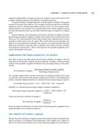
These views have important implications for the Phillips curve. In particular, they
imply that monetary policymakers face a long-run Phillips curve that is vertical, as
in Figure 33-3. If the Fed increases the money supply slowly, the inflation rate is
low, and the economy finds itself at point A. If the Fed increases the money supply
quickly, the inflation rate is high, and the economy finds itself at point B. In either
case, the unemployment rate tends toward its normal level, called the natural rate
of unemployment. The vertical long-run Phillips curve illustrates the conclusion that
unemployment does not depend on money growth and inflation in the long run.
The vertical long-run Phillips curve is, in essence, one expression of the classi-
cal idea of monetary neutrality. As you may recall, we expressed this idea in Chap-
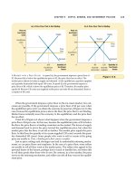
ter 31 with a vertical long-run aggregate-supply curve. Indeed, as Figure 33-4
illustrates, the vertical long-run Phillips curve and the vertical long-run aggregate-
supply curve are two sides of the same coin. In panel (a) of this figure, an increase
in the money supply shifts the aggregate-demand curve to the right from AD
1

financial economist at Keycorp, a Cleve-
land bank, “at a time when revenue
growth is constrained.”
But with unemployment already at a
low 5.5 percent and the economy looking
stronger than expected this summer,
more analysts are worried that it may be
only a matter of time before wage pres-
sures begin to build again as they did in
the late 1980s. . . .
The labor shortages are wide-
spread and include both skilled and
unskilled jobs. Among the hardest oc-
cupations to fill are computer analyst
and programmer, aerospace engineer,
construction trades worker, and various
types of salespeople. But even fast
food establishments in the St. Louis
area and elsewhere have resorted to
signing bonuses as well as premium pay
and more generous benefits to attract
applicants. . . .
So far, upward pressure on pay is
relatively modest, a phenomenon that
economists say is surprising in light of an
uninterrupted business expansion that is
now five and a half years old.
“We have less wage pressure
than, historically, anyone would have
guessed,” said Stuart G. Hoffman, chief

economist at PNC Bank in Pittsburgh.
But wages have already crept up
a bit and could accelerate even if the
economy slackens from its recent rapid
growth pace. And if the economy
maintains significant momentum, some
analysts say, all bets are off. If growth
continues another six months at above
2.5 percent or so, Mark Zandi, chief
economist for Regional Financial Associ-
ates, said, “we’ll be looking at wage infla-
tion right square in the eye.” . . .
[
Author’s note:
In fact, wage inflation did
rise. The rate of increase in compensation
per hour paid by U.S. businesses rose
from 1.8 percent in 1994 to 4.4 percent in
1998. But thanks to a fall in world com-
modity prices and a surge in productivity
growth, higher wage inflation didn’t trans-
late into higher price inflation. A case
study later in this chapter considers these
events in more detail.]
One worker who has taken advan-
tage of the current environment is Clyde
Long, a thirty-year-old who switched jobs
to join Trinity Packaging in May. He had
been working about two miles away at
Ross Industries, which makes food-

processing equipment, and quit without
having anything else lined up.
In a week, Mr. Long had hired on at
Trinity where, as a press operator, he now
earns $8.55 an hour—$1.25 more than at
his old job—with better benefits and train-
ing as well. “It’s a whole lot better here,”
he said.
SOURCE: The New York Times, September 5, 1996,
p. D1.
768 PART TWELVE SHORT-RUN ECONOMIC FLUCTUATIONS
to AD
2
. As a result of this shift, the long-run equilibrium moves from point A to
point B. The price level rises from P
1
to P
2
, but because the aggregate-supply curve
is vertical, output remains the same. In panel (b), more rapid growth in the money
supply raises the inflation rate by moving the economy from point A to point B.
But because the Phillips curve is vertical, the rate of unemployment is the same at
these two points. Thus, the vertical long-run aggregate-supply curve and the ver-
tical long-run Phillips curve both imply that monetary policy influences nominal
variables (the price level and the inflation rate) but not real variables (output and
unemployment). Regardless of the monetary policy pursued by the Fed, output
and unemployment are, in the long run, at their natural rates.
What is so “natural” about the natural rate of unemployment? Friedman and
Phelps used this adjective to describe the unemployment rate toward which the
economy tends to gravitate in the long run. Yet the natural rate of unemployment

is not necessarily the socially desirable rate of unemployment. Nor is the natural
rate of unemployment constant over time. For example, suppose that a newly
formed union uses its market power to raise the real wages of some workers above
the equilibrium level. The result is a surplus of workers and, therefore, a higher
natural rate of unemployment. This unemployment is “natural” not because it is
good but because it is beyond the influence of monetary policy. More rapid money
growth would not reduce the market power of the union or the level of unem-
ployment; it would lead only to more inflation.
Although monetary policy cannot influence the natural rate of unemploy-
ment, other types of policy can. To reduce the natural rate of unemployment,
policymakers should look to policies that improve the functioning of the labor
market. Earlier in the book we discussed how various labor-market policies, such
as minimum-wage laws, collective-bargaining laws, unemployment insurance,
and job-training programs, affect the natural rate of unemployment. A policy
change that reduced the natural rate of unemployment would shift the long-run
Unemployment
Rate
0 Natural rate of
unemployment
Inflation
Rate
B
Long-run
Phillips curve
High
inflation
Low
inflation
A
2. . . . but unemployment

remains at its natural rate
in the long run.
1. When the
Fed increases
the growth rate
of the money
supply, the
rate of inflation
increases . . .
Figure 33-3
THE LONG-RUN PHILLIPS CURVE.
According to Friedman and
Phelps, there is no tradeoff
between inflation and
unemployment in the long run.
Growth in the money supply
determines the inflation rate.
Regardless of the inflation
rate, the unemployment rate
gravitates toward its natural
rate. As a result, the long-run
Phillips curve is vertical.
CHAPTER 33 THE SHORT-RUN TRADEOFF BETWEEN INFLATION AND UNEMPLOYMENT 769
Phillips curve to the left. In addition, because lower unemployment means more
workers are producing goods and services, the quantity of goods and services
supplied would be larger at any given price level, and the long-run aggregate-
supply curve would shift to the right. The economy could then enjoy lower unem-
ployment and higher output for any given rate of money growth and inflation.
EXPECTATIONS AND THE SHORT-RUN PHILLIPS CURVE
At first, the denial by Friedman and Phelps of a long-run tradeoff between infla-

tion and unemployment might not seem persuasive. Their argument was based on
an appeal to theory. By contrast, the negative correlation between inflation and un-
employment documented by Phillips, Samuelson, and Solow was based on data.
Why should anyone believe that policymakers faced a vertical Phillips curve when
the world seemed to offer a downward-sloping one? Shouldn’t the findings of
Phillips, Samuelson, and Solow lead us to reject the classical conclusion of mone-
tary neutrality?
Quantity
of Output
Natural rate
of output
Natural rate of
unemployment
0
Price
Level
P
2
P
1
Aggregate
demand,
AD
1

Long-run aggregate
supply
Long-run Phillips
curve
(a) The Model of Aggregate Demand and Aggregate Supply

Unemployment
Rate
0
Inflation
Rate
(b) The Phillips Curve
2. . . . raises
the price
level . . .
1. An increase in
the money supply
increases aggregate
demand . . .
B
A
AD
2
B
A
4. . . . but leaves output and unemployment
at their natural rates.
3. . . . and
increases the
inflation rate . . .
Figure 33-4
H
OW THE LONG-RUN PHILLIPS CURVE IS RELATED TO THE MODEL OF AGGREGATE
D
EMAND AND AGGREGATE SUPPLY. Panel (a) shows the model of aggregate demand and
aggregate supply with a vertical aggregate-supply curve. When expansionary monetary

policy shifts the aggregate-demand curve to the right from AD
1
to AD
2
, the equilibrium
moves from point A to point B. The price level rises from P
1
to P
2
, while output remains
the same. Panel (b) shows the long-run Phillips curve, which is vertical at the natural
rate of unemployment. Expansionary monetary policy moves the economy from
lower inflation (point A) to higher inflation (point B) without changing the rate of
unemployment.
770 PART TWELVE SHORT-RUN ECONOMIC FLUCTUATIONS
Friedman and Phelps were well aware of these questions, and they offered
a way to reconcile classical macroeconomic theory with the finding of a down-
ward-sloping Phillips curve in data from the United Kingdom and the United
States. They claimed that a negative relationship between inflation and unem-
ployment holds in the short run but that it cannot be used by policymakers in the
long run. In other words, policymakers can pursue expansionary monetary policy
to achieve lower unemployment for a while, but eventually unemployment re-
turns to its natural rate, and more expansionary monetary policy leads only to
higher inflation.
Friedman and Phelps reasoned as we did in Chapter 31 when we explained
the difference between the short-run and long-run aggregate-supply curves. (In
fact, the discussion in that chapter drew heavily on the legacy of Friedman and
Phelps.) As you may recall, the short-run aggregate-supply curve is upward
sloping, indicating that an increase in the price level raises the quantity of goods
and services that firms supply. By contrast, the long-run aggregate-supply curve is

vertical, indicating that the price level does not influence quantity supplied in the
long run. Chapter 31 presented three theories to explain the upward slope of
the short-run aggregate-supply curve: misperceptions about relative prices,
sticky wages, and sticky prices. Because perceptions, wages, and prices adjust to
changing economic conditions over time, the positive relationship between the
price level and quantity supplied applies in the short run but not in the long
run. Friedman and Phelps applied this same logic to the Phillips curve. Just as
the aggregate-supply curve slopes upward only in the short run, the tradeoff
between inflation and unemployment holds only in the short run. And just as
the long-run aggregate-supply curve is vertical, the long-run Phillips curve is
also vertical.
To help explain the short-run and long-run relationship between inflation and
unemployment, Friedman and Phelps introduced a new variable into the analysis:
expected inflation. Expected inflation measures how much people expect the overall
price level to change. As we discussed in Chapter 31, the expected price level af-
fects the perceptions of relative prices that people form and the wages and prices
that they set. As a result, expected inflation is one factor that determines the posi-
tion of the short-run aggregate-supply curve. In the short run, the Fed can take ex-
pected inflation (and thus the short-run aggregate-supply curve) as already
determined. When the money supply changes, the aggregate-demand curve shifts,
and the economy moves along a given short-run aggregate-supply curve. In the
short run, therefore, monetary changes lead to unexpected fluctuations in output,
prices, unemployment, and inflation. In this way, Friedman and Phelps explained
the Phillips curve that Phillips, Samuelson, and Solow had documented.
Yet the Fed’s ability to create unexpected inflation by increasing the money
supply exists only in the short run. In the long run, people come to expect what-
ever inflation rate the Fed chooses to produce. Because perceptions, wages, and
prices will eventually adjust to the inflation rate, the long-run aggregate-supply
curve is vertical. In this case, changes in aggregate demand, such as those due to
changes in the money supply, do not affect the economy’s output of goods and

services. Thus, Friedman and Phelps concluded that unemployment returns to its
natural rate in the long run.
The analysis of Friedman and Phelps can be summarized in the following
equation (which is, in essence, another expression of the aggregate-supply equa-
tion we saw in Chapter 31):
CHAPTER 33 THE SHORT-RUN TRADEOFF BETWEEN INFLATION AND UNEMPLOYMENT 771
ϭϪa
΂
Ϫ
΃
.
This equation relates the unemployment rate to the natural rate of unemployment,
actual inflation, and expected inflation. In the short run, expected inflation is
given. As a result, higher actual inflation is associated with lower unemployment.
(How much unemployment responds to unexpected inflation is determined by the
size of a, a number that in turn depends on the slope of the short-run aggregate-
supply curve.) In the long run, however, people come to expect whatever inflation
the Fed produces. Thus, actual inflation equals expected inflation, and unemploy-
ment is at its natural rate.
This equation implies there is no stable short-run Phillips curve. Each short-
run Phillips curve reflects a particular expected rate of inflation. (To be precise, if
you graph the equation, you’ll find that the short-run Phillips curve intersects the
long-run Phillips curve at the expected rate of inflation.) Whenever expected in-
flation changes, the short-run Phillips curve shifts.
According to Friedman and Phelps, it is dangerous to view the Phillips curve
as a menu of options available to policymakers. To see why, imagine an economy
at its natural rate of unemployment with low inflation and low expected inflation,
shown in Figure 33-5 as point A. Now suppose that policymakers try to take ad-
vantage of the tradeoff between inflation and unemployment by using monetary
or fiscal policy to expand aggregate demand. In the short run when expected in-

flation is given, the economy goes from point A to point B. Unemployment falls be-
low its natural rate, and inflation rises above expected inflation. Over time, people
get used to this higher inflation rate, and they raise their expectations of inflation.
When expected inflation rises, firms and workers start taking higher inflation into
Expected
inflation
Actual
inflation
Natural rate of
unemployment
Unemployment
rate
Unemployment
Rate
0 Natural rate of
unemployment
Inflation
Rate
C
B
Long-run
Phillips curve
A
Short-run Phillips curve
with high expected
inflation
Short-run Phillips curve
with low expected
inflation
1. Expansionary policy moves

the economy up along the
short-run Phillips curve . . .
2. . . . but in the long run, expected
inflation rises, and the short-run
Phillips curve shifts to the right.
Figure 33-5
HOW EXPECTED INFLATION
SHIFTS THE SHORT-RUN
PHILLIPS CURVE
. The higher the
expected rate of inflation, the
higher the short-run tradeoff
between inflation and
unemployment. At point A,
expected inflation and actual
inflation are both low, and
unemployment is at its natural
rate. If the Fed pursues an
expansionary monetary policy,
the economy moves from point A
to point B in the short run. At
point B, expected inflation is still
low, but actual inflation is high.
Unemployment is below its
natural rate. In the long run,
expected inflation rises, and the
economy moves to point C. At
point C, expected inflation and
actual inflation are both high,
and unemployment is back

to its natural rate.
772 PART TWELVE SHORT-RUN ECONOMIC FLUCTUATIONS
account when setting wages and prices. The short-run Phillips curve then shifts to
the right, as shown in the figure. The economy ends up at point C, with higher in-
flation than at point A but with the same level of unemployment.
Thus, Friedman and Phelps concluded that policymakers do face a tradeoff be-
tween inflation and unemployment, but only a temporary one. If policymakers use
this tradeoff, they lose it.
THE NATURAL EXPERIMENT
FOR THE NATURAL-RATE HYPOTHESIS
Friedman and Phelps had made a bold prediction in 1968: If policymakers try to
take advantage of the Phillips curve by choosing higher inflation in order to re-
duce unemployment, they will succeed at reducing unemployment only tem-
porarily. This view—that unemployment eventually returns to its natural rate,
regardless of the rate of inflation—is called the natural-rate hypothesis. A few
years after Friedman and Phelps proposed this hypothesis, monetary and fiscal
policymakers inadvertently created a natural experiment to test it. Their labora-
tory was the U.S. economy.
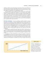
Before we see the outcome of this test, however, let’s look at the data that
Friedman and Phelps had when they made their prediction in 1968. Figure 33-6
shows the unemployment rate and the inflation rate for the period from 1961 to
1968. These data trace out a Phillips curve. As inflation rose over these eight years,
unemployment fell. The economic data from this era seemed to confirm the trade-
off between inflation and unemployment.
The apparent success of the Phillips curve in the 1960s made the prediction of
Friedman and Phelps all the more bold. In 1958 Phillips had suggested a negative
natural-rate hypothesis
the claim that unemployment
eventually returns to its normal,
or natural, rate, regardless of

the rate of inflation
Unemployment
Rate (percent)
Inflation Rate
(percent per year)
1968
1966
1961
1962
1963
1967
1965
1964
123456789100
2
4
6
8
10
Figure 33-6
THE PHILLIPS CURVE
IN THE
1960S. This figure uses
annual data from 1961 to 1968 on
the unemployment rate and on
the inflation rate (as measured by
the GDP deflator) to show the
negative relationship between
inflation and unemployment.
SOURCE: U.S. Department of Labor;

U.S. Department of Commerce.
CHAPTER 33 THE SHORT-RUN TRADEOFF BETWEEN INFLATION AND UNEMPLOYMENT 773
association between inflation and unemployment. In 1960 Samuelson and Solow
had showed it existed in U.S. data. Another decade of data had confirmed the re-
lationship. To some economists at the time, it seemed ridiculous to claim that the
Phillips curve would break down once policymakers tried to use it.
But, in fact, that is exactly what happened. Beginning in the late 1960s, the
government followed policies that expanded the aggregate demand for goods and
services. In part, this expansion was due to fiscal policy: Government spending
rose as the Vietnam War heated up. In part, it was due to monetary policy: Because
the Fed was trying to hold down interest rates in the face of expansionary fiscal
policy, the money supply (as measured by M2) rose about 13 percent per year dur-
ing the period from 1970 to 1972, compared to 7 percent per year in the early 1960s.
As a result, inflation stayed high (about 5 to 6 percent per year in the late 1960s and
early 1970s, compared to about 1 to 2 percent per year in the early 1960s). But, as
Friedman and Phelps had predicted, unemployment did not stay low.
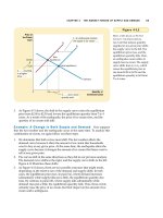
Figure 33-7 displays the history of inflation and unemployment from 1961 to
1973. It shows that the simple negative relationship between these two variables
started to break down around 1970. In particular, as inflation remained high in the
early 1970s, people’s expectations of inflation caught up with reality, and the un-
employment rate reverted to the 5 percent to 6 percent range that had prevailed in
the early 1960s. Notice that the history illustrated in Figure 33-7 closely resembles
the theory of a shifting short-run Phillips curve shown in Figure 33-5. By 1973,
policymakers had learned that Friedman and Phelps were right: There is no trade-
off between inflation and unemployment in the long run.
QUICK QUIZ: Draw the short-run Phillips curve and the long-run Phillips
curve. Explain why they are different.
Unemployment
Rate (percent)
Inflation Rate

(percent per year)
1973
1966
1972
1971
1961
1962
1963
1967
1968
1969
1970
1965
1964
123456789100
2
4
6
8
10
Figure 33-7
THE BREAKDOWN OF
THE
PHILLIPS CURVE. This
figure shows annual data
from 1961 to 1973 on the
unemployment rate and on the
inflation rate (as measured by
the GDP deflator). Notice that the
Phillips curve of the 1960s breaks

down in the early 1970s.
SOURCE: U.S. Department of Labor;
U.S. Department of Commerce.
774 PART TWELVE SHORT-RUN ECONOMIC FLUCTUATIONS
SHIFTS IN THE PHILLIPS CURVE:
THE ROLE OF SUPPLY SHOCKS
Friedman and Phelps had suggested in 1968 that changes in expected inflation
shift the short-run Phillips curve, and the experience of the early 1970s convinced
most economists that Friedman and Phelps were right. Within a few years,
INTHE1960S AND 1970S, POLICYMAKERS
learned that high expected inflation
shifts the short-run Phillips curve out-
ward, making actual inflation more
likely. In the 1990s, the opposite oc-
curred, as expected inflation fell and
helped keep actual inflation low.
The Virtuous Circle
of Low Inflation
BY JACOB M. SCHLESINGER
Why does inflation remain so low?
Some experts credit greater cor-
porate efficiency. Others cite a growing
labor force. Luck, in the form of cheap oil
and a strong dollar, helps. But the raging
economic debate often overlooks one
simple answer: because inflation remains
so low. In other words, it isn’t just a mat-
ter of mathematical formulas such as a
Phillips-curve tradeoff between inflation
and jobs; it also is the nebulous matter of

mass psychology. The economy may be
entering a phase in which low inflation is
no longer considered a lucky, transitory
phenomenon but an integral part of its
fabric. And if enough executives, suppli-
ers, consumers and workers believe it
will last, they will act in ways that help
make it last.
“For the past couple of years, peo-
ple were expecting inflation to rise, but
it hasn’t,” says Janet Yellen, the chief
White House economist and former Fed-
eral Reserve governor. “Slowly, people
are being convinced that inflation is
down and it’s going to stay down,
[which] is helpful in keeping inflation
down. Inflationary expectations feed
directly into wage bargaining and price
setting.”
This substantial exorcising of the
inflationary specter flows partly from
the Fed’s new credibility: a widespread
belief that it is committed to keeping
prices relatively stable and knows how to
do so. . . .
A widely cited measure of public
attitudes, the University of Michigan’s
Survey of Consumers, is reflecting two
significant changes this year, says
Richard Curtin, its director. First, long-

term inflation expectations—the pre-
dicted annual inflation rate for the next
five to 10 years—have slipped below
3% for the first time since the survey
began asking the question nearly two
decades ago. Second, long-term inflation
expectations now nearly equal short-
term expectations. . . .
This outlook eases inflationary pres-
sures in many ways. Recall the 1970s,
Ms. Yellen says, “when expectations of
future inflation led workers to demand
wage increases that would compensate
them for expected inflation, and firms to
give wage increases believing they could
pass on price increases.” . . .
“In the 1970s and 1980s, we had
price increases baked into our projec-
tions,” says Warren L. Batts, chairman
of both Premark International Inc. and
Tupperware Corp. and head of the
National Association of Manufacturers.
“We thought we could charge our cus-
tomers [more], and therefore we could
pay our suppliers. [Now], you know you
can’t charge, so you don’t pay.”
Of course, inflationary fears aren’t
completely cured, as last week’s stock
and bond market jitters show. Rampant
inflation in the 1970s shattered the no-

tion that America was immune to the
problem. Remaining traces of apprehen-
sion may not be all bad. “The moment
we become complacent about infla-
tion,” says Deputy Treasury Secretary
Lawrence Summers, “is the moment we
will start to have an inflation problem.”
SOURCE: The Wall Street Journal, August 18, 1997,
p. A1.
IN THE NEWS
The Benefits of Low
Expected Inflation