Tài liệu 39 Auditory Psychophysics for Coding Applications pdf
Bạn đang xem bản rút gọn của tài liệu. Xem và tải ngay bản đầy đủ của tài liệu tại đây (414.98 KB, 28 trang )
Jenkins, W. K. “Auditory Psychophysics for Coding Applications”
Digital Signal Processing Handbook
Ed. Vijay K. Madisetti and Douglas B. Williams
Boca Raton: CRC Press LLC, 1999
c
1999 by CRC Press LLC
Hall, J.L. “Auditory Psychophysics for Coding Applications”
Digital Signal Processing Handbook
Ed. Vijay K. Madisetti and Douglas B. Williams
Boca Raton: CRC Press LLC, 1999
c
1999 by CRC Press LLC
39
Auditory Psychophysics for Coding
Applications
39.1 Introduction
39.2 Definitions
Loudness • Pitch • Threshold of Hearing • Differential Threshold • Masked Threshold • Critical Bands and Peripheral Auditory Filters
39.3 Summary of Relevant Psychophysical Data
Joseph L. Hall
Bell Laboratories
Lucent Technologies
Loudness • Differential Thresholds • Masking
39.4 Conclusions
References
In this chapter we review properties of auditory perception that are relevant to the
design of coders for acoustic signals. The chapter begins with a general definition
of a perceptual coder, then considers what the “ideal” psychophysical model would
consist of and what use a coder could be expected to make of this model. We then
present some basic definitions and concepts. The chapter continues with a review of
relevant psychophysical data, including results on threshold, just-noticeable differences,
masking, and loudness. Finally, we attempt to summarize the present state of the art,
the capabilities and limitations of present-day perceptual coders for audio and speech,
and what areas most need work.
39.1
Introduction
A coded signal differs in some respect from the original signal. One task in designing a coder is to
minimize some measure of this difference under the constraints imposed by bit rate, complexity,
or cost. What is the appropriate measure of difference? The most straightforward approach is to
minimize some physical measure of the difference between original and coded signal. The designer
might attempt to minimize RMS difference between the original and coded waveform, or perhaps
the difference between original and coded power spectra on a frame-by-frame basis. However, if the
purpose of the coder is to encode acoustic signals that are eventually to be listened to1 by people,
1 Perceptual coding is not limited to speech and audio. It can be applied also to image and video [16]. In this paper we
consider only coders for acoustic signals.
c
1999 by CRC Press LLC
these physical measures do not directly address the appropriate issue. For signals that are to be
listened to by people, the “best” coder is the one that sounds the best. There is a very clear distinction
between physical and perceptual measures of a signal (frequency vs. pitch, intensity vs. loudness,
for example). A perceptual coder can be defined as a coder that minimizes some measure of the
difference between original and coded signal so as to minimize the perceptual impact of the coding
noise. We can define the best coder given a particular set of constraints as the one in which the coding
noise is least objectionable.
It follows that the designer of a perceptual coder needs some way to determine the perceptual
quality of a coded signal. “Perceptual quality” is a poorly defined concept, and it will be seen that in
some sense it cannot be uniquely defined. We can, however, attempt to provide a partial answer to
the question of how it can be determined. We can present something of what is known about human
auditory perception from psychophysical listening experiments and show how these phenomena
relate to the design of a coder.
One requirement for successful design of a perceptual coder is a satisfactory model for the signaldependent sensitivity of the auditory system. Present-day models are incomplete, but we can attempt
to specify what the properties of a complete model would be. One possible specification is that, for
any given waveform (the signal), it accurately predicts the loudness, as a function of pitch and of time,
of any added waveform (the noise). If we had such a complete model, then we would in principle
be able to build a transparent coder, defined as one in which the coded signal is indistinguishable
from the original signal, or at least we would be able to determine whether or not a given coder
was transparent. It is relatively simple to design a psychophysical listening experiment to determine
whether the coding noise is audible, or equivalently, whether the subject can distinguish between
original and coded signal. Any subject with normal hearing could be expected to give similar results
to this experiment. While present-day models are far from complete, we can at least describe the
properties of a complete model.
There is a second requirement that is more difficult to satisfy. This is the need to be able to determine
which of two coded samples, each of which has audible coding noise, is preferable. While a satisfactory
model for the signal-dependent sensitivity of the auditory system is in principle sufficient for the
design of a transparent coder, the question of how to build the best nontransparent coder does not
have a unique answer. Often, design constraints preclude building a transparent coder. Even the best
coder built under these constraints will result in audible coding noise, and it is under some conditions
impossible to specify uniquely how best to distribute this noise. One listener may prefer the more
intelligible version, while another may prefer the more natural sounding version. The preferences
of even a single listener might very well depend on the application. In the absence of any better
criterion, we can attempt to minimize the loudness of the coding noise, but it must be understood
that this is an incomplete solution.
Our purpose in this paper is to present something of what is known about human auditory
perception in a form that may be useful to the designer of a perceptual coder. We do not attempt
to answer the question of how this knowledge is to be utilized, how to build a coder. Present-day
perceptual coders for the most part utilize a feedforward paradigm: analysis of the signal to be coded
produces specifications for allowable coding noise. Perhaps a more general method is a feedback
paradigm, in which the perceptual model somehow makes possible a decision as to which of two
coded signals is “better”. This decision process can then be iterated to arrive at some optimum solution.
It will be seen that for proper exploitation of some aspects of auditory perception the feedforward
paradigm may be inadequate and the potentially more time-consuming feedback paradigm may be
required. How this is to be done is part of the challenge facing the designer.
c
1999 by CRC Press LLC
39.2
Definitions
In this section we define some fundamental terms and concepts and clarify the distinction between
physical and perceptual measures.
39.2.1
Loudness
When we increase the intensity of a stimulus its loudness increases, but that does not mean that
intensity and loudness are the same thing. Intensity is a physical measure. We can measure the
intensity of a signal with an appropriate measuring instrument, and if the measuring instrument
is standardized and calibrated correctly anyone else anywhere in the world can measure the same
signal and get the same result. Loudness is perceptual magnitude. It can be defined as “that attribute
of auditory sensation in terms of which sounds can be ordered on a scale extending from quiet to
loud” ([23], p.47). We cannot measure it directly. All we can do is ask questions of a subject and
from the responses attempt to infer something about loudness. Furthermore, we have no guarantee
that a particular stimulus will be as loud for one subject as for another. The best we can do is assume
that, for a particular stimulus, loudness judgments for one group of normal-hearing people will be
similar to loudness judgments for another group.
There are two commonly used measures of loudness. One is loudness level (unit phon) and the
other is loudness (unit sone). These two measures differ in what they describe and how they are
obtained. The phon is defined as the intensity, in dB SPL, of an equally loud 1-kHz tone. The sone
is defined in terms of subjectively measured loudness ratios. A stimulus half as loud as a one-sone
stimulus has a loudness of 0.5 sones, a stimulus ten times as loud has a loudness of 10 sones, etc. A
1-kHz tone at 40 dB SPL is arbitrarily defined to have a loudness of one sone.
The argument can be made that loudness matching, the procedure used to obtain the phon scale,
is a less subjective procedure than loudness scaling, the procedure used to obtain the sone scale. This
argument would lead to the conclusion that the phon is the more objective of the two measures and
that the sone is more subject to individual variability. This argument breaks down on two counts:
first, for dissimilar stimuli even the supposedly straightforward loudness-matching task is subject to
large and poorly understood order and bias effects that can only be described as subjective. While
loudness matching of two equal-frequency tone bursts generally gives stable and repeatable results,
the task becomes more difficult when the frequencies of the two tone bursts differ. Loudness matching
between two dissimilar stimuli, as for example between a pure tone and a multicomponent complex
signal, is even more difficult and yields less stable results. Loudness-matching experiments have to be
designed carefully, and results from these experiments have to be interpreted with caution. Second,
it is possible to measure loudness in sones, at least approximately, by means of a loudness-matching
procedure. Fletcher [6] states that under some conditions loudness adds. Binaural presentation of a
stimulus results in loudness doubling; and two equally-loud stimuli, far enough apart in frequency
that they do not mask each other, are twice as loud as one. If loudness additivity holds, then it follows
that the sone scale can be generated by matching loudness of a test stimulus to binaural stimuli or
to pairs of tones. This approach must be treated with caution. As Fletcher states, “However, this
method [scaling] is related more directly to the scale we are seeking (the sone scale) than the two
preceding ones (binaural or monaural loudness additivity)” ([6], p. 278). The loudness additivity
approach relies on the assumption that loudness summation is perfect, and there is some more recent
evidence [28, 33] that loudness summation, at least for binaural vs. monaural presentation, is not
perfect.
c
1999 by CRC Press LLC
39.2.2
Pitch
The American Standards Association defines pitch as “that attribute of auditory sensation in which
sounds may be ordered on a musical scale”. Pitch bears much the same relationship to frequency
as loudness does to intensity: frequency is an objective physical measure, while pitch is a subjective
perceptual measure. Just as there is not a one-to-one relationship between intensity and loudness, so
also there is not a one-to-one relationship between frequency and pitch. Under some conditions, for
example, loudness can be shown to decrease with decreasing frequency with intensity held constant,
and pitch can be shown to decrease with increasing intensity with frequency held constant ([40], p.
409).
39.2.3
Threshold of Hearing
Since the concept of threshold is basic to much of what follows, it is worthwhile at this point to
discuss it in some detail. It will be seen that thresholds are determined not only by the stimulus and
the observer but also by the method of measurement. While this discussion is phrased in terms of
threshold of hearing, much of what follows applies as well to differential thresholds (just-noticeable
differences) discussed in the next subsection.
By the simplest definition, the threshold of hearing (equivalently, auditory threshold) is the lowest
intensity that the listener can hear. This definition is inadequate because we cannot directly measure
the listener’s perception. A first-order correction, therefore, is that the threshold of hearing is the
lowest intensity that elicits from the listener the response that the sound is audible. Given this
definition, we can present a stimulus to the listener and ask whether he or she can hear it. If we
do this, we soon find that identical stimuli do not always elicit identical responses. In general, the
probability of a positive response increases with increasing stimulus intensity and can be described
by a psychometric function such as that shown for a hypothetical experiment in Fig. 39.1. Here the
stimulus intensity (in dB) appears on the abscissa and the probability P (C) of a positive response
appears on the ordinate. The yes-no experiment could be described by a psychometric function that
ranges from zero to one, and threshold could be defined as the stimulus intensity that elicits a positive
response in 50% of the trials.
FIGURE 39.1: Idealized psychometric functions for hypothetical yes-no experiment (zero to one)
and for hypothetical two-interval forced-choice experiment (0.5 to one).
c
1999 by CRC Press LLC
A difficulty with the simple yes-no experiment is that we have no control over the subject’s criterion
level. The subject may be using a strict criterion (“yes” only if the signal is definitely present) or a lax
criterion (“yes” if the signal might be present). The subject can respond correctly either by a positive
response in the presence of a stimulus (hit) or by a negative response in the absence of a stimulus
(correct rejection). Similarly the subject can respond incorrectly either by a negative response in the
presence of a stimulus (miss) or by a positive response in the absence of a stimulus (false alarm).
Unless the experimenter is willing to use an elaborate and time-consuming procedure that involves
assigning rewards to correct responses and penalties to incorrect responses, the criterion level is
uncontrolled.
The field of psychophysics that deals with this complication is called detection theory. The field of
psychophysical detection theory is highly developed [12] and a complete description is far beyond
the scope of this paper. Very briefly, the subject’s response is considered to be based on an internal
decision variable, a random variable drawn from a distribution with mean and standard deviation
that depend on the stimulus. If we assume that the decision variable is normally distributed with a
fixed standard deviation σ and a mean that depends only on stimulus intensity, then we can define
an index of sensitivity d for a given stimulus intensity as the difference between m0 (the mean in
the absence of the stimulus) and ms (the mean in the presence of the stimulus), divided by σ . An
ideal observer (a hypothetical subject who does the best possible job for the task at hand) gives a
positive response if and only if the decision variable exceeds an internal criterion level. An increase
in criterion level decreases the probability of a false alarm and increases the probability of a miss.
A simple and satisfactory way to deal with the problem of uncontrolled criterion level is to use a
criterion-free experimental paradigm. The simplest is perhaps the two-interval forced choice (2IFC)
paradigm, in which the stimulus is presented at random in one of two observation intervals. The
subject’s task is to determine which of the two intervals contained the stimulus. The ideal observer
selects the interval that elicits the larger decision variable, and criterion level is no longer a factor.
Now the subject has a 50% chance of choosing the correct interval even in the absence of any stimulus,
so the psychometric function goes from 0.5 to 1.0 as shown in Fig. 39.1. A reasonable definition of
threshold is P (C) = 0.75, halfway between the chance level of 0.5 and one. If the decision variable is
normally distributed with a fixed standard deviation, it can be shown that this definition of threshold
corresponds to a d of 0.95.
The number of intervals can be increased beyond two. In this case, the ideal observer responds
correctly if the decision variable for the interval containing the stimulus is larger than the largest of
the N-1 decision variables for the intervals not containing the stimulus. A common practice is, for
an N-interval forced choice paradigm (NIFC), to define threshold as the point halfway between the
chance level of 1/N and one. This is a perfectly acceptable practice so long as it is recognized that the
measured threshold is influenced by the number of alternatives. For a 3IFC paradigm this definition
of threshold corresponds to a d of 1.12 and for a 4IFC paradigm it corresponds to a d of 1.24.
39.2.4
Differential Threshold
The differential threshold is conceptually similar to the auditory threshold discussed above, and many
of the same comments apply. The differential threshold, or just-noticeable difference (JND), is the
amount by which some attribute of a signal has to change in order for the observer to be able to
detect the change. A tone burst, for example, can be specified in terms of frequency, intensity, and
duration, and a differential threshold for any of these three attributes can be defined and measured.
The first attempt to provide a quantitative description of differential thresholds was provided by
the German physiologist E. H. Weber in the first half of the 19th century. According to Weber’s law,
the just-noticeable difference I is proportional to the stimulus intensity I , or I /I = K, where the
constant of proportionality I /I is known as the Weber fraction. This was supposed to be a general
description of sensitivity to changes of intensity for a variety of sensory modalities, not limited just
c
1999 by CRC Press LLC
to hearing, and it has since been applied to perception of nonintensive variables such as frequency.
It was recognized at an early stage that this law breaks down at near-threshold intensities, and in the
latter half of the 19th century the German physicist G. T. Fechner suggested the modification that is
now known as the modified Weber law, I /(I + I0 ) = K, where I0 is a constant. While Weber’s law
provides a reasonable first-order description of intensity and frequency discrimination in hearing,
in general it does not hold exactly, as will be seen below.
As with the threshold of hearing, the differential threshold can be measured in different ways, and
the result depends to some extent on how it is measured. The simplest method is a same-different
paradigm, in which two stimuli are presented and the subject’s task is to judge whether or not they
are the same. This method suffers from the same drawback as the yes-no paradigm for auditory
threshold: we do not have control over the subject’s criterion level.
If the physical attribute being measured is simply related to some perceptual attribute, then the
differential threshold can be measured by requiring the subject to judge which of two stimuli has
more of that perceptual attribute. A just-noticeable difference for frequency, for example, could be
measured by requiring the subject to judge which of two stimuli is of higher pitch; or a just noticeable
difference for intensity could be measured by requiring the subject to judge which of two stimuli is
louder. As with the 2IFC paradigm discussed above for auditory threshold, this method removes the
problem of uncontrolled criterion level.
There are more general methods that do not assume a knowledge of the relationship between
the physical attribute being measured and a perceptual attribute. The most useful, perhaps, is the
N-interval forced choice method: N stimuli are presented, one of which differs from the other N-1
along the dimension being measured. The subject’s task is to specify which one of the N stimuli is
different from the other N-1.
Note that there is a close parallel between the differential threshold and the auditory threshold
described in the previous subsection. The auditory threshold can be regarded as a special case of the
just-noticeable difference for intensity, where the question is by how much the intensity has to differ
from zero in order to be detectable.
39.2.5
Masked Threshold
The masked threshold of a signal is defined as the threshold of that signal (the probe) in the presence
of another signal (the masker). A related term is masking, which is the elevation of threshold of the
probe by the masker: it is the difference between masked and absolute threshold. More generally,
the reduction of loudness of a supra-threshold signal is also referred to as masking. It will be seen
that masking can appear in many forms, depending on spectral and temporal relationships between
probe and masker.
Many of the comments that applied to measurement of absolute and differential thresholds also
apply to measurement of masked threshold. The simplest method is to present masker plus probe
and ask the subject whether or not the probe is present. Once again there is a problem with criterion
level. Another method is to present stimuli in two intervals and ask the subject which one contains
the probe. This method can give useful results but can, under some conditions, give misleading
results. Suppose, for example, that the probe and masker are both pure tones at 1 kHz, but that the
two signals are 180◦ out of phase. As the intensity of the probe is increased from zero, the intensity
of the composite signal will first decrease, then increase. The two signals, masker alone and masker
plus probe, may be easily distinguishable, but in the absence of additional information the subject
has no way of telling which is which.
A more robust method for measuring masked threshold is the N-interval forced choice method
described above, in which the subject specifies which of the N stimuli differs from the other N-1.
Subjective percepts in masking experiments can be quite complex and can differ from one observer
to another. In the N-interval forced choice method the observer has the freedom to base judgments
c
1999 by CRC Press LLC
on whatever attribute is most easily detected, and it is not necessary to instruct the observer what to
listen for.
Note that the differential threshold for intensity can be regarded as a special case of the masked
threshold in which the probe is an intensity-scaled version of the masker.
A note on terminology: suppose two signals, x1 (t) and [x1 (t) + x2 (t)] are just distinguishable.
If x2 (t) is a scaled version of x1 (t), then we are dealing with intensity discrimination. If x1 (t) and
x2 (t) are two different signals, then we are dealing with masking, with x1 (t) the masker and x2 (t)
the probe. In either case, the difference can be described in several ways. These ways include (1) the
intensity increment between x1 (t) and [x1 (t) + x2 (t)], I ; (2) the intensity increment relative to
x1 (t), I /I ; (3) the intensity ratio between x1 (t) and [x1 (t) + x2 (t)], (I + I )/I ; (4) the intensity
increment in dB, 10 × log10 ( I /I ); and (5) the intensity ratio in dB, 10 × log10 [(I + I )/I ]. These
ways are equivalent in that they show the same information, although for a particular application
one way may be preferable to another for presentation purposes. Another measure that is often used,
particularly in the design of perceptual coders, is the intensity of the probe x2 (t). This measure is
subject to misinterpretation and must be used with caution. Depending on the coherence between
x1 (t) and x2 (t), a given probe intensity can result in a wide range of intensity increments I . The
resulting ambiguity has been responsible for some confusion.
39.2.6
Critical Bands and Peripheral Auditory Filters
The concepts of critical bands and peripheral auditory filters are central to much of the auditory
modeling work that is used in present-day perceptual coders. Scharf, in a classic review article [33],
defines the empirical critical bandwidth as “that bandwidth at which subjective responses rather
abruptly change”. Simply put, for some psychophysical tasks the auditory system behaves as if it
consisted of a bank of bandpass filters (the critical bands) followed by energy detectors. Examples of
critical-band behavior that are particularly relevant for the designer of a coder include the relationship
between bandwidth and loudness (Fig. 39.5) and the relationship between bandwidth and masking
(Fig. 39.10). Another example of critical-band behavior is phase sensitivity: in experiments measuring the detectability of amplitude and of frequency modulation, the auditory system appears to be
sensitive to the relative phase of the components of a complex sound only so long as the components
are within a critical band [9, 45].
The concept of the critical band was introduced more than a half-century ago by Fletcher [6], and
since that time it has been studied extensively. Fletcher’s pioneering contribution is ably documented
by Allen [1], and Scharf ’s 1970 review article [33] gives references to some later work. More recently,
Moore and his co-workers have made extensive measurements of peripheral auditory filters [24].
The value of critical bandwidths has been the subject of some discussion, because of questions
of definition and method of measurement. Figure 39.2 ([31], Fig. 1) shows critical bandwidth as a
function of frequency for Scharf ’s empirical definition (the bandwidth at which subjective responses
undergo some sort of change). Results from several experiments are superimposed here, and they
are in substantial agreement with each other. Moore and Glasberg [26] argue that the bandwidths
shown in Fig. 39.2 are determined not only by the bandwidth of peripheral auditory filters but also
by changes in processing efficiency. By their argument, the bandwidth of peripheral auditory filters
is somewhat smaller than the values shown in Fig. 39.2 at frequencies above 1 kHz and substantially
smaller, by as much as an octave, at lower frequencies.
39.3
Summary of Relevant Psychophysical Data
In Section 39.2, we introduced some basic concepts and definitions. In this section, we review some
relevant psychophysical results. There are several excellent books and book chapters that have been
c
1999 by CRC Press LLC
FIGURE 39.2: Empirical critical bandwidth. (Source: Scharf, B., Critical bands, ch. 5 in Foundations
of Modern Auditory Theory, Vol. 1, Tobias, J.V., ed., Academic Press, NY, 1970. With permission).
written on this subject, and we have neither the space nor the inclination to duplicate material found
in these other sources. Our attempt here is to make the reader aware of some relevant results and to
refer him or her to sources where more extensive treatments may be found.
39.3.1
Loudness
Loudness Level and Frequency
For pure tones, loudness depends on both intensity and frequency. Figure 39.3 (modified
from [37], p. 124) shows loudness level contours. The curves are labeled in phons and, in parentheses,
sones. These curves have been remeasured many times since, with some variation in the results, but
the basic conclusions remain unchanged. The most sensitive region is around 2-3 kHz. The lowfrequency slope of the loudness level contours is flatter at high loudness levels than at low. It follows
that loudness level grows more rapidly with intensity at low frequencies than at high. The 38- and
48-phon contours are (by definition) separated by 10 dB at 1 kHz, but they are only about 5 dB apart
at 100 Hz.
This figure also shows contours that specify the dynamic range of hearing. Tones below the 8-phon
contour are inaudible, and tones above the dotted line are uncomfortable. The dynamic range of
hearing, the distance between these two contours, is greatest around 2 to 3 kHz and decreases at
lower and higher frequencies. In practice, the useful dynamic range is substantially less. We know
today that extended exposure to sounds at much lower levels than the dotted line in Fig. 39.3 can
result in temporary or permanent damage to the ear. It has been suggested that extended exposure
to sounds as low as 70 to 75 dB(A) may produce permanent high-frequency threshold shifts in some
c
1999 by CRC Press LLC
individuals [39].
FIGURE 39.3: Loudness level contours. Parameters: phons (sones). The bottom curve (8 phons)
is at the threshold of hearing. The dotted line shows Wegel’s 1932 results for “threshold of feeling”.
This line is many dB above levels that are known today to produce permanent damage to the auditory
system. (Modified from Stevens, S.S. and Davis, H.W., Hearing, John Wiley & Sons, New York, 1938).
Loudness and Intensity
Figure 39.4 (modified from [32], Fig. 5) shows loudness growth functions, the relationship
between stimulus intensity in dB SPL and loudness in sones, for tones of different frequencies. As
can be seen in Fig. 39.4, the loudness growth function depends on frequency. Above about 40 dB SPL
for a 1-kHz tone the relationship is approximately described by the power law L(I ) = (I /I0 )1/3 , so
that if the intensity I is increased by 9 dB the loudness L is approximately doubled.2 The relationship
between loudness and intensity has been modeled extensively [1, 6, 46].
Loudness and Bandwidth
The loudness of a complex sound of fixed intensity, whether a tone complex or a band of noise,
depends on its bandwidth, as is shown in Fig. 39.5 ([48], Fig. 3). For sounds well above threshold,
the loudness remains more or less constant so long as the bandwidth is less than a critical band. If the
bandwidth is greater than a critical band, the loudness increases with increasing bandwidth. Near
threshold the trend is reversed, and the loudness decreases with increasing bandwidth.3
2 This power-law relationship between physical and perceptual measures of a stimulus was studied in great detail by S. S.
Stevens. This relationship is now commonly referred to as Stevens’ Law. Stevens measured exponents for many sensory
modalities, ranging from a low of 0.33 for loudness and brightness to a high of 3.5 for electric shock produced by a 60-Hz
electric current delivered to the skin.
3 These data were obtained by comparing the loudness of a single 1-kHz tone and the loudness of a four-tone complex of
the specified bandwidth centered at 1 kHz. The systematic difference between results when the tone was adjusted (“T”
c
1999 by CRC Press LLC
FIGURE 39.4: Loudness growth functions. (Modified from Scharf, B., Loudness, ch. 6 in Handbook
of Perception, Vol. IV, Hearing, Carterette, E.C. and Friedman M.P., eds., Academic Press, New York,
1978. With permission).
These phenomena have been modeled successfully by utilizing the loudness growth functions
shown in Fig. 39.4 in a model that calculates total loudness by summing the specific loudness per
critical band [49]. The loudness growth function is very steep near threshold, so that dividing the
total energy of the signal into two or more critical bands results in a reduction of total loudness. The
loudness growth function well above threshold is less steep, so that dividing the total energy of the
signal into two or more critical bands results in an increase of total loudness.
Loudness and Duration
Everything we have talked about so far applies to steady-state, long-duration stimuli. These
results are reasonably well understood and can be modeled reasonably well by present-day models.
However, there is a host of psychophysical data having to do with aspects of temporal structure of
the signal that are less well understood and less well modeled. The subject of temporal dynamics of
auditory perception is an area where there is a great deal of room for improvement in models for
perceptual auditory coders. One example of this subject is the relationship between loudness and
duration discussed here. Other examples appear in a later section on temporal aspects of masking.
There is general agreement that, for fixed intensity, loudness increases with duration up to stimulus
durations of a few hundred milliseconds. (Other factors, usually discussed under the terms adaptation
symbol) and when the complex was adjusted (“C” symbol) is an example of the bias effects mentioned in section 39.2.1
(Loudness).
c
1999 by CRC Press LLC
FIGURE 39.5: Loudness vs. bandwidth of tone complex. (Source: Zwicker, E. et al., Critical
bandwidth in loudness summation, J. Acoust. Soc. Am., 29: 548-557, 1957. With permission).
FIGURE 39.6: Frequency JND as a function of frequency and intensity (Modified from Wier, C.C.
et al., Frequency discrimination as a function of frequency and sensation level, J. Acoust. Soc. Am.,
61: 178-184, 1977. With permission).
c
1999 by CRC Press LLC
or fatigue, come into play for longer durations of many seconds or minutes. We will not discuss these
factors here.) The duration below which loudness increases with increasing duration is sometimes
referred to as the critical duration. Scharf [32] provides an excellent summary of studies of the
relationship between loudness and duration. In his survey, he cites values of critical duration ranging
from 10 msec to over 500 msec. About half the studies in Scharf ’s survey show that the total energy
(intensity x duration) stays constant below the critical duration for constant loudness, while the
remaining studies are about evenly split between total energy increasing and total energy decreasing
with increasing duration.
One possible explanation for this confused state of affairs is the inherent difficulty of making
loudness matches between dissimilar stimuli, discussed above in Section 39.2.1 (Loudness). Two
stimuli of different durations differ by more than “loudness”, and depending on a variety of poorlyunderstood experimental or individual factors what appears to be the same experiment may yield
different results in different laboratories or with different subjects.
Some support for this explanation comes from the fact that studies of threshold intensity as a
function of duration are generally in better agreement with each other than studies of loudness as a
function of duration. As discussed above in Section 39.2.3 (Threshold of Hearing) measurements
of auditory threshold depend to some extent on the method of measurement, but it is still possible
to establish an internally-consistent criterion-free measure. The exact results depend to some extent
on signal frequency, but there is reasonable agreement among various studies that total energy at
threshold remains approximately constant between about 10 msec and 100 msec. (See [41] for a
survey of studies of threshold intensity as a function of duration.)
39.3.2
Differential Thresholds
Frequency
Figure 39.6 shows frequency JND as a function of frequency and intensity as measured in
the most recent comprehensive study [43]. The frequency JND generally increases with increasing
frequency and decreases with increasing intensity, ranging from about 1 Hz at low frequency and
moderate intensity to more than 100 Hz at high frequency and low intensity.
The results shown in Fig. 39.6 are in basic agreement with results from most other studies of frequency JND’s with the exception of the earliest comprehensive study, by Shower and Biddulph ([43],
p. 180). Shower and Biddulph [35] found a more gradual increase of frequency JND with frequency.
As we have noted above, the results obtained in experiments of this nature are strongly influenced by
details of the method of measurement. Shower and Biddulph measured detectability of frequency
modulation of a pure tone; most other experimenters measured the ability of subjects to correctly
identify whether one tone burst was of higher or lower frequency than another. Why this difference
in procedure should produce this difference in results, or even whether this difference in procedure
is solely responsible for the difference in results, is unclear.
The Weber fraction f/f , where f is the frequency JND, is smallest at mid frequencies, in the
region from 500 Hz to 2 kHz. It increases somewhat at lower frequencies, and it increases very
sharply at high frequencies above about 4 kHz. Wier et al. [43] in their Fig. 1, reproduced here as
√
our Fig. 39.6, plotted log f against f . They found that this choice of axes resulted in the closest
fit to a straight line. It is not clear that this choice of axes has any theoretical basis; it appears simply
to be a choice that happens to work well. There have been extensive attempts to model frequency
selectivity. These studies suggest that the auditory system uses the timing of individual nerve impulses
at low frequencies, but that at high frequencies above a few kHz this timing information is no longer
available and the auditory system relies exclusively on place information from the mechanically tuned
inner ear.
Rosenblith and Stevens [30] provide an interesting example of the interaction between method of
c
1999 by CRC Press LLC
measurement and observed result. They compared frequency JNDs using two methods. One was
an “AX” method, in which the subject judged whether the second of a pair of tone bursts was of
higher or lower frequency than the first of the pair. The other was an “ABX” method, in which the
subject judged whether the third of three tone bursts, at the same frequency as one of the first two
tone bursts, was more similar to the first or to the second burst. They found that frequency JNDs
measured using the AX method were approximately half the size of frequency JNDs measured using
the ABX method, and they concluded that “... it would be rather imprudent to postulate a “true” DL
(difference limen), or to infer the behavior of the peripheral organ from the size of a DL measured
under a given set of conditions”. They discussed their results in terms of information theory, an active
topic at the time, and were unable to reach any definite conclusion. An analysis of their results in
terms of detection theory, which at that time was in its infancy, predicts their results almost exactly.4
Intensity
The Weber fraction I /I for pure tones is not constant but decreases slightly as stimulus
intensity increases. This change has been termed the near miss to Weber’s law. In most studies, the
Weber fraction has been found to be independent of frequency. An exception is Riesz’s study [29],
in which the Weber fraction was at a minimum at approximately 2 kHz and increased at higher and
lower frequencies.
Typical results are summarized in Fig. 39.7 ([18], Fig. 4). The solid straight line is a good fit to
Jesteadt’s intensity JND data at frequencies from 200 Hz to 8 kHz. The Weber fraction decreases
from about 0.44 at 5 dB SL (decibels above threshold) to about 0.12 at 80 dB SL. These results are
in substantial agreement with most other studies with the exception of Riesz’s study. Riesz’s data are
shown in Fig. 39.7 as the curves identified by symbols. There is a larger change of intensity JND with
intensity, and the intensity JND depends on frequency.
There is an interesting parallel between the results for intensity JND and the results for frequency
JND. In both cases, results from most studies are in agreement with the exception of one study:
Shower and Biddulph for frequency JND, and Riesz for intensity JND. In both cases, most studies
measured the ability of subjects to correctly identify the difference between two tone bursts. Both
of the outlying studies measured, instead, the ability of subjects to identify modulation of a tone:
Shower and Biddulph used frequency modulation and Riesz used amplitude modulation. It appears
that a modulated continuous tone may give different results than a pair of tone bursts. Whether this
is a real effect, and, if it is, whether it is due to stimulus artifact or to properties of the auditory system,
is unclear. The subject merits further investigation.
The Weber fraction for wideband noise appears to be independent of intensity. Miller [21] measured detectability of intensity increments in wide-band noise and found that the Weber fraction
I /I was approximately constant at 0.099 above 30 dB SL. It increased below 30 dB SL, which led
Miller to revive Fechner’s modification of Weber’s law as discussed above in Section 39.2.4 (Differential Threshold).
39.3.3
Masking
No aspect of auditory psychophysics is more relevant to the design of perceptual auditory coders than
masking, since the basic objective is to use the masking properties of speech to hide the coding noise.
4 Assume RV’s A, B, and X are drawn independently from normal distributions with means m , m and m , respectively,
A
B
X
and equal standard deviations σ . √ can be shown that the relevant decision variable in the AX experiment has mean
It
mA − mX and standard √
deviation 2 × σ , while the relevant decision variable in the ABX experiment has mean mA − mB
and standard deviation 6 × σ , a value almost twice as large.
c
1999 by CRC Press LLC
FIGURE 39.7: Summary of intensity JNDs for pure tones. Jesteadt et al. [18] found that the Weber
fraction I /I was independent of frequency (straight line). Riesz [29], using a different procedure,
found a dependence (connected points). (Source: Jesteadt, W. et al., Intensity Discrimination as a
function of frequency and sensation level, J. Acoust. Soc. Am., 61: 169-177, 1977. With permission).
It will be seen that while we can use present-day knowledge of masking to great advantage, there is
still much to be learned about properties of masking if we are to fully exploit it. Since some of the
major unresolved problems in modeling masking are related to the relative bandwidth of masker and
probe, our approach here is to present masking in terms of this relative bandwidth.
Tone Probe, Tone Masker
At one time, perhaps because of the demonstrated power of the Fourier transform in the analysis
of linear time-invariant systems, the sine wave was considered to be the “natural” signal to be used in
studies of human hearing. Much of the earliest work on masking dealt with the masking of one tone
by another [42]. Typical results are shown in Fig. 39.8 ([3], Fig. 1). Similar results appear in Wegel
and Lane [42]. The abscissa is probe frequency and the ordinate is masking in dB, the elevation of
masked over absolute threshold (15 dB SPL for 400-Hz tone). Three curves are shown, for 400-Hz
maskers at 40, 60, and 80 dB SPL.
Masking is greatest for probe frequencies slightly above or below the masker frequency of 400 Hz.
Maximum probe-to-masker ratios are −19 dB for an 80 dB SPL masker (probe intensity elevated 46
dB above the absolute threshold of 15 dB SPL), −15 dB for a 60 dB SPL masker, and −14 dB for a 40
dB SPL masker.
Masking decreases as probe frequency gets closer to 400 Hz. The probe frequencies closest to 400
Hz are 397 and 403 Hz, and at these frequencies the threshold probe-to-masker ratio is −26 dB for
an 80 dB SPL masker, −23 dB for a 60 dB SPL masker, and −21 dB for a 40 dB SPL masker.
Masking also decreases as probe frequency gets further away from masker frequency. For the 40 dB
SPL masker this selectivity is nearly symmetric in log frequency, but as the masker intensity increases
the masking becomes more and more asymmetric so that the 400-Hz masker produces much more
masking at higher frequencies than at lower.
The irregularities seen near probe frequencies of 400, 800, and 1200 Hz are the result of interactions
between masker and probe. When masker and probe frequencies are close, beating results. Even when
c
1999 by CRC Press LLC
FIGURE 39.8: Masking of tones by a 400-Hz tone at 40, 60, and 80 dB SPL. (Source: Egan, J.P. and
Hake, H.W., On the masking pattern of a simple auditory stimulus, J. Acoust. Soc. Am., 22: 622-630,
1950).
their frequencies are far apart, nonlinear effects in the auditory system result in complex interactions.
These irregularities provided incentive to use narrow bands of noise, rather than pure tones, as
maskers.
Tone Probe, Noise Masker
Fletcher and Munson [8] were among the first to use bands of noise as maskers. Figure 39.9 ([3],
Fig. 2) shows typical results. The conditions are similar to those for Fig. 39.8 except that now the
masker is a band of noise 90 Hz wide centered at 410 Hz. The maximum probe-to-masker ratios
occur for probe frequencies slightly above the center frequency of the masker, and they are much
greater than they were for the tone maskers shown in Fig. 39.8. Maximum probe-to-masker ratios are
−4 dB for an 80 dB SPL masker and −3 dB for 60 and 40 dB SPL maskers. The frequency selectivity
and upward spread of masking seen in Fig. 39.8 appear in Fig. 39.9 as well, but the irregularities seen
at harmonics of the masker frequency are greatly reduced.
An important effect that occurs in connection with masking of a tone probe by a band of noise
is the relationship between masker bandwidth and amount of masking. This relationship can be
presented in many ways, but the results can be described to a reasonable degree of accuracy by saying
that noise energy within a narrow band of frequencies surrounding the probe contributes to masking
while noise energy outside this band of frequencies does not. This is one manifestation of the critical
band described in Section 39.2.6 (Critical Bands and Peripheral Auditory Filters).
Figure 39.10 ([2], Fig. 6) shows results from a series of experiments designed to determine the
widths of critical bands. We are most concerned here with the closed symbols and the associated solid
and dotted straight lines. These show an expanded and elaborated repeat of a test Fletcher reported
in 1940 to measure the width of critical bands, and the results shown here are similar to Fletcher’s
results ([7], Fig. 124). The closed symbols show threshold level of probe signals at frequencies
ranging from 500 Hz to 8 kHz in dB relative to the intensity of a masking band of noise centered at
the frequency of the test signal and with the bandwidth shown on the abscissa. The intensity of the
masking noise is 60 dB SPL per 1/3 octave. Note that for narrow-band maskers the probe-to-masker
c
1999 by CRC Press LLC
FIGURE 39.9: Masking of tones by a 90-Hz wide band of noise centered at 410 Hz at 40, 60, and 80
dB SPL (Source: Egan, J.P. and Hake, H.W., On the masking pattern of a simple auditory stimulus,
J. Acoust. Soc. Am., 22: 622-630, 1950).
ratio is nearly independent of bandwidth, while for wide-band maskers the probe-to-masker ratio
decreases at approximately 3 dB per doubling of bandwidth. This result indicates that above a certain
bandwidth, approximated in this figure as the intersection of the asymptotic narrow-band horizontal
line and the asymptotic wide-band sloping lines, noise energy outside of this band does not contribute
to masking.
The results shown in Fig. 39.10 are from only one of many studies of masking of pure tones by
noise bands of varying bandwidths that lead to similar conclusions. The list includes Feldtkeller and
Zwicker [5] and Greenwood [13]. Scharf [33] provides additional references.
Noise Probe, Tone or Noise Masker
Masking of bands of noise, either by tone or noise maskers, has received relatively little attention.
This is unfortunate for the designer who is concerned with masking wide-band coding noise. Masking
of noise by tones is touched on in Zwicker [47], but the earliest study that gives actual data points
appears to be Hellman [15]. The threshold probe-to-masker ratios for a noise probe approximately
one critical band wide were −21 dB for a 60 dB SPL masker and −28 dB for a 90 dB SPL masker.
Threshold probe-to-masker ratios for an octave-band probe were −55 dB for 1-kHz maskers at 80
and 100 dB SPL. A 1-kHz masker at 90 dB SPL produced practically no masking of a wide-band
probe.
Hall [34] measured threshold intensity for noise bursts one-half, one, and two critical bands wide
c
1999 by CRC Press LLC
FIGURE 39.10: Threshold level of probe signals from 500 Hz to 8 kHz relative to overall level of noise
masker at bandwidth shown on the abscissa. (Modified from Bos, C.E. and de Boer, E., Masking and
discrimination, J. Acoust. Soc. Am., 39: 708-715, 1966. With permission).
with various center frequencies in the presence of 80 dB SPL pure-tone maskers ranging from an
octave below to an octave above the center frequency. Figure 39.11 shows results for a critical-band
1-kHz probe. The threshold probe-to-masker ratio for a 1-kHz masker is −24 dB, in agreement with
Hellman’s results, and the figure shows the same upward spread of masking that appears in Figs. 39.8
and 39.9. (Note that in Figs. 39.8 and 39.9 the masker is fixed and the abscissa is probe frequency,
while in Fig. 39.11 the probe is fixed and the abscissa is masker frequency.) A tone below 1 kHz
produces more masking than a tone above 1 kHz.
Masking of noise by noise is confounded by the question of phase relationships between probe
and masker. If masker and probe are identical in bandwidth and phase, then as we saw in Section 39.2.5 (Masked Threshold) the masked threshold becomes identical to the differential threshold.
Miller’s [21] Weber fraction I /I of 0.099 for intensity discrimination of wide-band noise, phrased
in terms of intensity of the just-detectable increment, leads to a probe-to-masker ratio of −26.3 dB.
More recently, Hall [14] measured threshold intensity for various combinations of probe and
masker bandwidths. These experiments differ from earlier experiments in that phase relationships
between probe and masker were controlled: all stimuli were generated by adding together equalamplitude random phase sinusoidal components, and components common to probe and masker
had identical phase. Results for one subject are shown in Fig. 39.12. Masker bandwidth appears
on the abscissa, and the parameter is probe bandwidth: A ⇒ 0 Hz, B ⇒ 4 Hz, C ⇒ 16 Hz, and
D ⇒ 64 Hz. All stimuli were centered at 1 kHz and the overall intensity of the masker was 70 dB
SPL.
c
1999 by CRC Press LLC
FIGURE 39.11: Threshold intensity for a 923-1083 Hz band of noise masked by an 80-dB SPL tone
at the frequency shown on the abscissa. (Source: Schroeder, M.R. et al., Optimizing digital speech
coders by exploiting masking properties of the human ear, J. Acoust. Soc. Am., 66: 1647-1652, 1979.
With permission).
This figure differs from Figs. 39.8 through 39.11 in that the vertical scale shows intensity increment between masker alone and masker plus just-detectable probe rather than intensity of the
just-detectable probe, and the results look quite different. For all probe bandwidths shown, the
intensity increment varies only slightly so long as the masker is at least as wide as the probe. The
intensity increment decreases when the probe is wider than the masker.
Asymmetry of Masking
Inspection of Figs. 39.8– 39.11 reveals large variation of threshold probe-to-masker intensity
ratios depending on the relative bandwidth of probe and masker. Tone maskers produce threshold
probe-to-masker ratios of −14 to −26 dB for tone probes, depending on the intensity of the masker
and the frequency of the probe (Fig. 39.8), and threshold probe-to-masker ratios of −21 to −28 dB
for critical-band noise probes ([15]; also Fig. 39.11). On the other hand, a tone masked by a band of
noise is audible only at much higher probe-to-masker ratios, in the neighborhood of 0 dB (Figs. 39.9
and 39.10). This asymmetry of masking (the term is due to Hellman, [15]) is of central importance in
the design of perceptual coders because of the different masking properties of noise-like and tone-like
portions of the coded signal [19]. Current perceptual models do not handle this asymmetry well, so
it is a subject we must examine closely.
The logical conclusion to be drawn from the numbers in the preceding paragraph at first appears
to be that a band of noise is a better masker than a tone, for both noise and tone probes. In fact, the
correct conclusion may be completely different. It can be argued that so long as the masker bandwidth
is at least as wide as the probe bandwidth, tones or bands of noise are equally effective maskers and
the psychophysical data can be described satisfactorily by current energy-based perceptual models,
properly applied. It is only when the bandwidth of the probe is greater than the bandwidth of the
masker that energy-based models break down and some criterion other than average energy must be
applied.
Figure 39.13 shows Egan and Hake’s results for 80 dB SPL tone and noise maskers superimposed
on each other. Results for the tone masker are shown as a solid curve and results for the noise masker
are shown as a dashed curve. (These curves are not identical to the corresponding curves in Figs. 39.8
and 39.9: They are average results from five subjects, while Figs. 39.8 and 39.9 were for a single
c
1999 by CRC Press LLC
FIGURE 39.12: Intensity increment between masker alone and masker plus just-detectable probe.
Probe bandwidth 0 Hz (A); 4 Hz (B); 16 Hz (C); 64 Hz (D). Frequency components common to probe
and masker have identical phase. (Source: Hall, J.L., Asymmetry of masking revisited: generalization
of masker and probe bandwidth, J. Acoust. Soc. Am., 101: 1023–1033, 1997. With permission).
subject.) The maximum amount of masking produced by the band of noise is 61 dB, while the tone
masker produces only 37 dB of masking for a 397-Hz probe.
The difference between tone and noise maskers may be more apparent than real, and for masking of
a tone the auditory system may be similarly affected by tone and noise maskers. What is plotted in this
figure is the elevation in threshold intensity of the probe tone by the masker, but the discrimination
the subject makes is in fact between masker alone and masker plus probe. As was discussed above
in Section 39.2.5 (Masked Threshold), since coherence between tone probe and masker depends on
the bandwidth of the masker, a probe tone of a given intensity can produce a much greater change in
intensity of probe plus masker for a tone masker than for a noise masker.
The stimulus in the Egan and Hake experiment with a 400-Hz masker and a 397-Hz probe is
identical to the stimulus Riesz used to measure intensity JND (see Section 47 Differential Thresholds:
Intensity, above). As Egan and Hake observe “... When the frequency of the masked stimulus is 397
or 403 c.p.s. [Hz], the amount of masking is evidently determined by the value of the differential
threshold for intensity at 400 c.p.s.” ([3], p. 624). Specifically, for the results shown in Fig. 39.13, the
threshold intensity of a 397-Hz tone is 52 dB SPL. This leads to a Weber fraction I /I (power at
envelope maximum minus power at envelope minimum, divided by power at envelope minimum)
of 0.17, which is only slightly higher than values obtained by Riesz and by Jesteadt et al. shown in
Fig. 39.7.
The situation with noise masker is more difficult to analyze because of the random nature of the
masker. The effective intensity increment between masker alone and masker plus probe depends on
the phase relationship between probe and 400-Hz component of the masker, which are uncontrolled
in the Egan and Hake experiment, and also on the effective time constant and bandwidth of the
analyzing auditory filter, which are unknown. However, for the experiment shown in Fig. 39.12 the
maskers were computer-generated repeatable stimuli, so that the intensity of masker plus probe could
be computed. The results shown in Fig. 39.12 lead to a Weber fraction I /I of 0.15 for tone masked
by tone and 0.10 for tone masked by 64-Hz wide noise. Results are similar for noise masked by noise,
so long as the masker is at least as wide as the probe. Weber fractions for the 64-Hz wide masker in
Fig. 39.12 range from 0.18 for a 4-Hz wide probe to 0.15 for a 64-Hz wide probe.
Our understanding of the factors leading to the results shown in Fig. 39.12 is obviously very limited,
but these results appear to be consistent with the view that to a first-order approximation the relevant
variable for masking is the Weber fraction I /I , the intensity of masker plus probe relative to the
c
1999 by CRC Press LLC
FIGURE 39.13: Masking produced by a 400-Hz masker at 80 dB SPL and a 90-Hz wide band of
noise centered at 410 Hz. (Source: Egan, J.P. and Hake, H.W., On the masking pattern of a simple
auditory stimulus, J. Acoust. Soc. Am., 22: 622-630, 1950).
intensity of the masker, so long as the masker is at least as wide as the probe. This is true for both tone
and noise maskers. Because of changes in coherence between probe and masker as masker bandwidth
changes, the corresponding probe intensity at threshold can be much lower for a tone masker than
for a probe masker, as is shown in Fig. 39.13.
The asymmetry that Hellman was primarily concerned with in her 1972 paper is the striking
difference between the threshold of a band of noise masked by a tone and of a tone masked by a band
of noise. It appears that this is a completely different effect than the asymmetry shown in Fig. 39.13
and one that cannot be accounted for by current energy-based models of masking. The difference
between the −5 to +5 dB threshold probe-to-masker ratios seen in Figs. 39.9 and 39.10 for tones
masked by noise and the −21 to −28 dB threshold probe-to-masker ratios for noise masked by tone
reported by Hellman and seen in Fig. 39.11 is due in part to the random nature of the noise masker
and to the change in coherence between masker and probe that we have already discussed. Even
when these factors are controlled, as in Fig. 39.12, decrease of masker bandwidth for a 64-Hz wide
band of noise results in a decrease of threshold intensity increment. (The situation is complicated by
the possibility of off-frequency listening. As we have already seen, neither a tone nor a noise masker
masks remote frequencies effectively. The 64-Hz band is narrow enough that off-frequency listening
is not a factor.) These and similar results lead to the conclusion that present-day models operating on
signal power are inadequate and that some envelope-based measure, such as the envelope maximum
or ratio of envelope maximum to minimum, must be considered [10, 11, 38].
Temporal Aspects of Masking
Up until now, we have discussed masking effects with simultaneous masker and probe. In order
to be able to deal effectively with a dynamically varying signal such as speech, we need to consider
nonsimultaneous masking as well. When the probe follows the masker, the effect is referred to as
forward masking. When the masker follows the probe, it is referred to as backward masking. Effects
have also been measured with a brief probe near the beginning or the end of a longer-duration masker.
These effects have been referred to as forward or backward fringe masking, respectively ([44], p. 162).
The various kinds of simultaneous and non-simultaneous masking are nicely illustrated in
c
1999 by CRC Press LLC
FIGURE 39.14: Masking of tone by ongoing wide-band noise with silent interval of 25, 50, 200, or
500 msec. This figure shows simultaneous, forward, backward, forward fringe, and backward fringe
masking. (Source: Elliott, L.L., Masking of tones before, during, and after brief silent periods in
noise, J. Acoust. Soc. Am., 45: 1277-1279, 1969. With permission).
Fig. 39.14 ([4], Fig. 1). The masker was wideband noise at an overall level of 70 dB SPL and the probe
was a brief 1.9-kHz tone burst. The masker was on continuously except for a silent interval of 25, 50,
200, or 500 msec. beginning at the 0-msec point on the abscissa. The four sets of data points show
thresholds for probes presented at various times relative to the gap for the four gap durations. Probe
thresholds in silence and in continuous noise are indicated on the ordinate by the symbols “Q” and
“CN”.
Forward masking appears as the gradual drop of probe threshold over a duration of more than
100 msec following the cessation of the masker. Backward masking appears as the abrupt increase
of masking, over a duration of a few tens of msec, immediately before the reintroduction of the
masker. Forward fringe masking appears as the more than 10-dB overshoot of masking immediately
following the reintroduction of the masker, and backward fringe masking appears as the smaller
overshoot immediately preceding the cessation of the masker. Backward masking is an important
effect for the designer of coders for acoustic signals because of its relationship to audibility of preecho. It is a puzzling effect, because it is caused by a masker that begins only after the probe has been
presented. Stimulus-related electrophysiological events can be recorded in the cortex several tens
of msec after presentation of the stimulus, so there may be some physiological basis for backward
masking. It is an unstable effect, and there is some evidence that backward masking decreases with
practice [20], ([23], p. 119).
Forward masking is a more robust effect, and it has been studied extensively. It is a complex
function of stimulus parameters, and we do not have a comprehensive model that predicts amount
of forward masking as a function of frequency, intensity, and time course of masker and of probe.
The following two examples illustrate some of its complexity.
Figure 39.15 ([17], Fig. 1) is from a study of the effects of masker frequency and intensity on forward
c
1999 by CRC Press LLC
FIGURE 39.15: Forward masking with identical masker and probe frequencies, as a function of
frequency, delay, and masker level (Source: Jesteadt, W. et al., Forwarding masking as a function of
frequency, masker level, and signal delay, J. Acoust. Soc. Am., 71: 950-962, 1982. With permission).
masking. Masker and probe were of the same frequency. The left and right columns show the same
data, plotted on the left against probe delay with masker intensity as a parameter and plotted on the
right against masker intensity with probe delay as a parameter. The amount of masking depends
in an orderly way on masker frequency, masker intensity, and probe delay. Jesteadt et al. were
able to fit these data with a single equation with three free constants. This equation, with minor
modification, was later found to give a satisfactory fit to data obtained with forward masking by
wide-band noise [25].
Striking effects can be observed when probe and masker frequencies differ. Figure 39.16 (modified
from [22], Fig. 8) superimposes simultaneous (open symbols) and forward (filled symbols) masking
curves for a 6-kHz probe at 36 dB SPL, 10 dB above the absolute threshold of 26 dB SPL. Rather than
showing the amount of masking for a fixed masker, this figure shows masker level, as a function of
masker frequency, sufficient to just mask the probe. It is clear that simultaneous and forward masking
differ, and that the difference depends on the relative frequency of masker and probe. Results such
as those shown in Fig. 39.16 are of interest to the field of auditory physiology because of similarities
between forward masking results and frequency selectivity of primary auditory neurons.
c
1999 by CRC Press LLC
FIGURE 39.16: Simultaneous (open symbols) and forward (closed symbols) masking of a 6-kHz
probe tone at 36 dB SPL. Masker frequency appears on the abscissa, and masker intensity just sufficient
to mask the probe appears on the abscissa. (Modified from Moore, B.C.J., Psychophysical tuning
curves measured in simultaneous and forward masking, J. Acoust. Soc. Am., 63: 524-532, 1978. With
permission).
39.4
Conclusions
Notwithstanding the successes obtained to date with perceptual coders for speech and audio [16, 19,
27, 36], there is still a great deal of room for further advancement. The most widely applied perceptual
models today apply an energy-based criterion to some critical-band transformation of the signal and
arrive at a prediction of acceptable coding noise. These models are essentially refinements of models
first described by Fletcher and his co-workers and further developed by Zwicker and others [34].
These models do a good job describing masking and loudness for steady-state bands of noise, but
they are less satisfactory for other signals. We can identify two areas in which there seem to be great
room for improvement. One of these areas presents a challenge jointly to the designer of coders and
to the auditory psychophysicist, and the other area presents a challenge primarily to the auditory
psychophysicist.
One area for additional research has to do with asymmetry of masking. Noise is a more effective
masker than tones, and this difference is not handled well by present-day perceptual models. Presentday coders first compute a measure of tonality of the signal and then use this measure empirically to
obtain an estimate of masking. This empirical approach has been applied successfully to a variety of
signals, but it is possible that an approach that is less empirical and more based on a comprehensive
model of auditory perception would be more robust.
As discussed in Section 39.3.3 (Masking: Asymmetry of Masking), there is evidence that there are
two separate factors contributing to this asymmetry of masking. The difference between noise and
tone maskers for narrow-band coding noise appears to result from problems with signal definition
rather than a difference in processing by the auditory system, and it may be that an effective way of
dealing with it will result not from an improved understanding of auditory perception but rather
from changes in the coder. A feedforward prediction of acceptable coding noise based on the energy
of the signal does not take into account phase relationships between signal and noise. What may be
required is a feedback, analysis-by-synthesis approach, in which a direct comparison is made between
the original signal and the proposed coded signal. This approach would require a more complex
encoder but leave the decoder complexity unchanged [27]. The difference between narrow-band
and wide-band coding noise, on the other hand, appears to call for a basic change in models of
c
1999 by CRC Press LLC