Tài liệu shi20396 chương 4 pdf
Bạn đang xem bản rút gọn của tài liệu. Xem và tải ngay bản đầy đủ của tài liệu tại đây (511.33 KB, 56 trang )
Chapter 4
4-1
1
R
C
R
A
R
B
R
D
C
A
B
W
D
1
2
3
R
B
R
A
W
R
B
R
C
R
A
2
1
W
R
A
R
Bx
R
Bx
R
By
R
By
R
B
2
1
1
Scale of
corner magnified
W
A
B
(e)
(f)
(d)
W
A
R
A
R
B
B
1
2
W
A
R
A
R
B
B
11
2
(a)
(b)
(c)
shi20396_ch04.qxd 8/18/03 10:35 AM Page 50
Chapter 4 51
4-2
(a)
R
A
= 2 sin 60 = 1.732
kN Ans.
R
B
= 2 sin 30 = 1
kN Ans.
(b)
S = 0.6
m
α = tan
−1
0.6
0.4 + 0.6
= 30.96
◦
R
A
sin 135
=
800
sin 30.96
⇒ R
A
= 1100
N Ans.
R
O
sin 14.04
=
800
sin 30.96
⇒ R
O
= 377
N Ans.
(c)
R
O
=
1.2
tan 30
= 2.078
kN Ans.
R
A
=
1.2
sin 30
= 2.4
kN Ans.
(d) Step 1: Find
R
A
and
R
E
h =
4.5
tan 30
= 7.794 m
ۗ
+
M
A
= 0
9R
E
− 7.794(400 cos 30) − 4.5(400 sin 30) = 0
R
E
= 400
N Ans.
F
x
= 0 R
Ax
+ 400 cos 30 = 0 ⇒ R
Ax
=−346.4N
F
y
= 0 R
Ay
+ 400 − 400 sin 30 = 0 ⇒ R
Ay
=−200 N
R
A
=
346.4
2
+ 200
2
= 400 N
Ans.
D
C
h
B
y
E
x
A
4.5 m
9 m
400 N
3
4
2
30°
60°
R
Ay
R
A
R
Ax
R
E
1.2 kN
60°
R
A
R
O
60°90°
30°
1.2 kN
R
A
R
O
45Њ Ϫ 30.96Њ ϭ 14.04Њ
135°
30.96°
30.96°
800 N
R
A
R
O
O
0.4 m
45°
800 N
␣
0.6 m
A
s
R
A
R
O
B
60°
90°
30°
2 kN
R
A
R
B
2
1
2 kN
60°
30°
R
A
R
B
shi20396_ch04.qxd 8/18/03 10:35 AM Page 51
52 Solutions Manual • Instructor’s Solution Manual to Accompany Mechanical Engineering Design
Step 2: Find components of
R
C
on link 4 and
R
D
ۗ
+
M
C
= 0
400(4.5) − (7.794 −1.9)R
D
= 0 ⇒ R
D
= 305.4N
Ans.
F
x
= 0 ⇒ (R
Cx
)
4
= 305.4N
F
y
= 0 ⇒ (R
Cy
)
4
=−400 N
Step 3: Find components of
R
C
on link 2
F
x
= 0
( R
Cx
)
2
+ 305.4 − 346.4 = 0 ⇒ (R
Cx
)
2
= 41 N
F
y
= 0
( R
Cy
)
2
= 200 N
4-3
(a)
ۗ
+
M
0
= 0
−18(60) + 14R
2
+ 8(30) − 4(40) = 0
R
2
= 71.43
lbf
F
y
= 0: R
1
− 40 + 30 + 71.43 − 60 = 0
R
1
=−1.43
lbf
M
1
=−1.43(4) =−5.72
lbf · in
M
2
=−5.72 − 41.43(4) =−171.44
lbf · in
M
3
=−171.44 − 11.43(6) =−240
lbf · in
M
4
=−240 + 60(4) = 0
checks!
4" 4" 6" 4"
Ϫ1.43
Ϫ41.43
Ϫ11.43
60
40 lbf 60 lbf
30 lbf
x
x
x
O
AB CD
y
R
1
R
2
M
1
M
2
M
3
M
4
O
V (lbf)
M
(lbf• in)
O
C
C
DB
A
B
D
E
305.4 N
346.4 N
305.4 N
41 N
400 N
200 N
400 N
200 N
400 N
Pin C
30°
305.4 N
400 N
400 N
200 N
41 N
305.4 N
200 N
346.4 N
305.4 N
(R
Cx
)
2
(R
Cy
)
2
C
B
A
2
400 N
4
R
D
(R
Cx
)
4
(R
Cy
)
4
D
C
E
Ans.
shi20396_ch04.qxd 8/18/03 10:35 AM Page 52
Chapter 4 53
(b)
F
y
= 0
R
0
= 2 + 4(0.150) = 2.6
kN
M
0
= 0
M
0
= 2000(0.2) + 4000(0.150)(0.425)
= 655 N · m
M
1
=−655 + 2600(0.2) =−135
N · m
M
2
=−135 + 600(0.150) =−45
N · m
M
3
=−45 +
1
2
600(0.150) = 0
checks!
(c)
M
0
= 0: 10R
2
− 6(1000) = 0 ⇒ R
2
= 600
lbf
F
y
= 0: R
1
− 1000 + 600 = 0 ⇒ R
1
= 400
lbf
M
1
= 400(6) = 2400
lbf · ft
M
2
= 2400 − 600(4) = 0
checks!
(d)
ۗ
+
M
C
= 0
−10R
1
+ 2(2000) + 8(1000) = 0
R
1
= 1200
lbf
F
y
= 0: 1200 − 1000 − 2000 + R
2
= 0
R
2
=
1800 lbf
M
1
= 1200(2) = 2400
lbf · ft
M
2
= 2400 + 200(6) = 3600
lbf · ft
M
3
= 3600 − 1800(2) = 0
checks!
2000 lbf
1000 lbf
R
1
O
O
M
1
M
2
M
3
R
2
6 ft 2 ft2 ft
AB
C
y
M
1200
Ϫ1800
200
x
x
x
6 ft 4 ft
A
O
O
O
B
Ϫ600
M
1
M
2
V (lbf)
1000 lbf
y
R
1
R
2
400
M
(lbf
•ft)
x
x
x
V (kN)
150 mm200 mm 150 mm
2.6
Ϫ655
M
(N• m)
0.6
M
1
M
2
M
3
2 kN
4 kN/m
y
A
O
O
O
O
BC
R
O
M
O
x
x
x
shi20396_ch04.qxd 8/18/03 10:35 AM Page 53
54 Solutions Manual • Instructor’s Solution Manual to Accompany Mechanical Engineering Design
(e) ۗ
+
M
B
= 0
−7R
1
+ 3(400) − 3(800) = 0
R
1
=−171.4
lbf
F
y
= 0: −171.4 − 400 + R
2
− 800 = 0
R
2
= 1371.4
lbf
M
1
=−171.4(4) =−685.7
lbf · ft
M
2
=−685.7 − 571.4(3) =−2400
lbf · ft
M
3
=−2400 + 800(3) = 0
checks!
(f) Break at A
R
1
= V
A
=
1
2
40(8) = 160
lbf
ۗ
+
M
D
= 0
12(160) − 10R
2
+ 320(5) = 0
R
2
= 352
lbf
F
y
= 0
−160 + 352 − 320 + R
3
= 0
R
3
= 128
lbf
M
1
=
1
2
160(4) = 320
lbf · in
M
2
= 320 −
1
2
160(4) = 0
checks! (hinge)
M
3
= 0 − 160(2) =−320
lbf · in
M
4
=−320 + 192(5) = 640
lbf · in
M
5
= 640 − 128(5) = 0
checks!
40 lbf/in
V (lbf)
O
O
160
Ϫ160
Ϫ128
192
M
320 lbf
160 lbf 352 lbf 128 lbf
M
1
M
2
M
3
M
4
M
5
x
x
x
8"
5"
2"
5"
40 lbf/in
160 lbf
O
A
y
BD
C
A
320 lbf
R
2
R
3
R
1
V
A
A
O
O
O
C
M
V (lbf )
800
Ϫ171.4
Ϫ571.4
3 ft 3 ft4 ft
800 lbf400 lbf
B
y
M
1
M
2
M
3
R
1
R
2
x
x
x
shi20396_ch04.qxd 8/18/03 10:35 AM Page 54
Chapter 4 55
4-4
(a)
q = R
1
x
−1
− 40x − 4
−1
+ 30x − 8
−1
+ R
2
x − 14
−1
− 60x − 18
−1
V = R
1
− 40x − 4
0
+ 30x − 8
0
+ R
2
x − 14
0
− 60x − 18
0
(1)
M = R
1
x − 40x − 4
1
+ 30x − 8
1
+ R
2
x − 14
1
− 60x − 18
1
(2)
for
x = 18
+
V = 0
and
M = 0
Eqs. (1) and (2) give
0 = R
1
− 40 + 30 + R
2
− 60 ⇒ R
1
+ R
2
= 70
(3)
0 = R
1
(18) − 40(14) + 30(10) + 4R
2
⇒ 9R
1
+ 2R
2
= 130
(4)
Solve (3) and (4) simultaneously to get
R
1
=−1.43
lbf,
R
2
= 71.43
lbf. Ans.
From Eqs. (1) and (2), at
x = 0
+
,
V = R
1
=−1.43
lbf,
M = 0
x = 4
+
: V =−1.43 − 40 =−41.43, M =−1.43x
x = 8
+
: V =−1.43 −40 + 30 =−11.43
M =−1.43(8) − 40(8 − 4)
1
=−171.44
x = 14
+
: V =−1.43 −40 + 30 + 71.43 = 60
M =−1.43(14) − 40(14 − 4) + 30(14 − 8) =−240
.
x = 18
+
: V = 0, M = 0
See curves of V and M in Prob. 4-3 solution.
(b)
q = R
0
x
−1
− M
0
x
−2
− 2000x − 0.2
−1
− 4000x − 0.35
0
+ 4000x − 0.5
0
V = R
0
− M
0
x
−1
− 2000x − 0.2
0
− 4000x − 0.35
1
+ 4000x − 0.5
1
(1)
M = R
0
x − M
0
− 2000x − 0.2
1
− 2000x − 0.35
2
+ 2000x − 0.5
2
(2)
at
x = 0.5
+
m,
V = M = 0
, Eqs. (1) and (2) give
R
0
− 2000 − 4000(0.5 − 0.35) = 0 ⇒ R
1
= 2600 N = 2.6
kN Ans.
R
0
(0.5) − M
0
− 2000(0.5 − 0.2) − 2000(0.5 − 0.35)
2
= 0
with
R
0
= 2600
N,
M
0
= 655
N · m Ans.
With R
0
and M
0
, Eqs. (1) and (2) give the same V and M curves as Prob. 4-3 (note for
V,
M
0
x
−1
has no physical meaning).
(c)
q = R
1
x
−1
− 1000x − 6
−1
+ R
2
x − 10
−1
V = R
1
− 1000x − 6
0
+ R
2
x − 10
0
(1)
M = R
1
x − 1000x − 6
1
+ R
2
x − 10
1
(2)
at
x = 10
+
ft,
V = M = 0
, Eqs. (1) and (2) give
R
1
− 1000 + R
2
= 0 ⇒ R
1
+ R
2
= 1000
10R
1
− 1000(10 − 6) = 0 ⇒ R
1
= 400 lbf
,
R
2
= 1000 − 400 = 600 lbf
0 ≤ x ≤ 6: V = 400 lbf, M = 400x
6 ≤ x ≤ 10: V = 400 −1000(x − 6)
0
= 600 lbf
M = 400x − 1000(x − 6) = 6000 − 600x
See curves of Prob. 4-3 solution.
shi20396_ch04.qxd 8/18/03 10:35 AM Page 55
56 Solutions Manual • Instructor’s Solution Manual to Accompany Mechanical Engineering Design
(d)
q = R
1
x
−1
− 1000x − 2
−1
− 2000x − 8
−1
+ R
2
x − 10
−1
V = R
1
− 1000x − 2
0
− 2000x − 8
0
+ R
2
x − 10
0
(1)
M = R
1
x − 1000x − 2
1
− 2000x − 8
1
+ R
2
x − 10
1
(2)
At
x = 10
+
,
V = M = 0
from Eqs. (1) and (2)
R
1
− 1000 − 2000 + R
2
= 0 ⇒ R
1
+ R
2
= 3000
10R
1
− 1000(10 − 2) − 2000(10 − 8) = 0 ⇒ R
1
= 1200 lbf
,
R
2
= 3000 − 1200 = 1800 lbf
0 ≤ x ≤ 2: V = 1200 lbf, M = 1200x lbf ·ft
2 ≤ x ≤ 8: V = 1200 −1000 = 200 lbf
M = 1200x − 1000(x − 2) = 200x + 2000 lbf · ft
8 ≤ x ≤ 10: V = 1200 − 1000 − 2000 =−1800 lbf
M = 1200x − 1000(x − 2) − 2000(x −8) =−1800x + 18 000 lbf · ft
Plots are the same as in Prob. 4-3.
(e)
q = R
1
x
−1
− 400x − 4
−1
+ R
2
x − 7
−1
− 800x − 10
−1
V = R
1
− 400x − 4
0
+ R
2
x − 7
0
− 800x − 10
0
(1)
M = R
1
x − 400x − 4
1
+ R
2
x − 7
1
− 800x − 10
1
(2)
at
x = 10
+
,
V = M = 0
R
1
− 400 + R
2
− 800 = 0 ⇒ R
1
+ R
2
= 1200
(3)
10R
1
− 400(6) + R
2
(3) = 0 ⇒ 10R
1
+ 3R
2
= 2400
(4)
Solve Eqs. (3) and (4) simultaneously:
R
1
=−171.4
lbf,
R
2
= 1371.4 lbf
0 ≤ x ≤ 4: V =−171.4 lbf, M =−171.4x lbf ·ft
4 ≤ x ≤ 7: V =−171.4 −400 =−571.4 lbf
M =−171.4x − 400(x − 4)
lbf · ft
=−571.4x + 1600
7 ≤ x ≤ 10: V =−171.4 − 400 + 1371.4 = 800 lbf
M =−171.4x − 400(x − 4) + 1371.4(x − 7) = 800x − 8000
lbf · ft
Plots are the same as in Prob. 4-3.
(f)
q = R
1
x
−1
− 40x
0
+ 40x − 8
0
+ R
2
x − 10
−1
− 320x − 15
−1
+ R
3
x − 20
V = R
1
− 40x + 40x − 8
1
+ R
2
x − 10
0
− 320x − 15
0
+ R
3
x − 20
0
(1)
M = R
1
x − 20x
2
+ 20x − 8
2
+ R
2
x − 10
1
− 320x − 15
1
+ R
3
x − 20
1
(2)
M = 0 at x = 8 in ∴
8R
1
− 20(8)
2
= 0 ⇒ R
1
= 160 lbf
at
x = 20
+
, V and M = 0
160 − 40(20) + 40(12) + R
2
− 320 + R
3
= 0 ⇒ R
2
+ R
3
= 480
160(20) − 20(20)
2
+ 20(12)
2
+ 10R
2
− 320(5) = 0 ⇒ R
2
= 352
lbf
R
3
= 480 − 352 = 128 lbf
0 ≤ x ≤ 8: V = 160 − 40x lbf, M = 160x −20x
2
lbf · in
8 ≤ x ≤ 10: V = 160 −40x + 40(x − 8) =−160 lbf
,
M = 160x − 20x
2
+ 20(x −8)
2
= 1280 − 160x lbf · in
shi20396_ch04.qxd 8/18/03 10:35 AM Page 56
Chapter 4 57
10 ≤ x ≤ 15: V = 160 −40x + 40(x −8) + 352 = 192 lbf
M = 160x − 20x
2
+ 20(x −8) + 352(x − 10) = 192x − 2240
15 ≤ x ≤ 20: V = 160 − 40x + 40(x −8) + 352 − 320 =−128 lbf
M = 160x − 20x
2
− 20(x −8) + 352(x − 10) − 320(x − 15)
=−128x + 2560
Plots of V and M are the same as in Prob. 4-3.
4-5 Solution depends upon the beam selected.
4-6
(a) Moment at center,
x
c
= (l − 2a)/2
M
c
=
w
2
l
2
(l − 2a) −
l
2
2
=
wl
2
l
4
− a
At reaction,
|M
r
|=wa
2
/2
a = 2.25, l = 10 in, w = 100
lbf/in
M
c
=
100(10)
2
10
4
− 2.25
= 125
lbf · in
M
r
=
100(2.25
2
)
2
= 253.1
lbf · in Ans.
(b) Minimum occurs when
M
c
=|M
r
|
wl
2
l
4
− a
=
wa
2
2
⇒ a
2
+ al − 0.25l
2
= 0
Taking the positive root
a =
1
2
−l +
l
2
+ 4(0.25l
2
)
=
l
2
√
2 − 1
= 0.2071l
Ans.
for l = 10 in and
w
= 100 lbf,
M
min
= (100/2)[(0.2071)(10)]
2
= 214.5
lbf · in
4-7 For the ith wire from bottom, from summing forces vertically
(a)
T
i
= (i + 1)W
From summing moments about point a,
M
a
= W(l − x
i
) − iWx
i
= 0
Giving,
x
i
=
l
i + 1
WiW
T
i
x
i
a
shi20396_ch04.qxd 8/18/03 10:35 AM Page 57
58 Solutions Manual • Instructor’s Solution Manual to Accompany Mechanical Engineering Design
So
W =
l
1 + 1
=
l
2
x =
l
2 + 1
=
l
3
y =
l
3 + 1
=
l
4
z =
l
4 + 1
=
l
5
(b) With straight rigid wires, the mobile is not stable. Any perturbation can lead to all wires
becoming collinear. Consider a wire of length l bent at its string support:
M
a
= 0
M
a
=
iWl
i + 1
cos α −
ilW
i + 1
cos β = 0
iWl
i + 1
(cos α −cos β) = 0
Moment vanishes when
α = β
for any wire. Consider a ccw rotation angle
β
, which
makes
α → α +β
and
β → α − β
M
a
=
iWl
i + 1
[cos(α +β) − cos(α − β)]
=
2iWl
i + 1
sin α sin β
.
=
2iWlβ
i + 1
sin α
There exists a correcting moment of opposite sense to arbitrary rotation
β
. An equation
for an upward bend can be found by changing the sign of
W
. The moment will no longer
be correcting. A curved, convex-upward bend of wire will produce stable equilibrium
too, but the equation would change somewhat.
4-8
(a)
C =
12 + 6
2
= 9
CD =
12 − 6
2
= 3
R =
3
2
+ 4
2
= 5
σ
1
= 5 + 9 = 14
σ
2
= 9 − 5 = 4
2
s
(12, 4
cw
)
C
R
D
2
1
1
2
2
p
(6, 4
ccw
)
y
x
cw
ccw
W
i
W
il
i ϩ 1
T
i

␣
l
i ϩ 1
shi20396_ch04.qxd 8/18/03 10:35 AM Page 58
Chapter 4 59
φ
p
=
1
2
tan
−1
4
3
= 26.6
◦
cw
τ
1
= R = 5, φ
s
= 45
◦
− 26.6
◦
= 18.4
◦
ccw
(b)
C =
9 + 16
2
= 12.5
CD =
16 − 9
2
= 3.5
R =
5
2
+ 3.5
2
= 6.10
σ
1
= 6.1 + 12.5 = 18.6
φ
p
=
1
2
tan
−1
5
3.5
= 27.5
◦
ccw
σ
2
= 12.5 − 6.1 = 6.4
τ
1
= R = 6.10
,
φ
s
= 45
◦
− 27.5
◦
= 17.5
◦
cw
(c)
C =
24 + 10
2
= 17
CD =
24 − 10
2
= 7
R =
7
2
+ 6
2
= 9.22
σ
1
= 17 + 9.22 = 26.22
σ
2
= 17 − 9.22 = 7.78
2
s
(24, 6
cw
)
C
R
D
2
1
1
2
2
p
(10, 6
ccw
)
y
x
cw
ccw
x
12.5
12.5
6.10
17.5Њ
x
6.4
18.6
27.5Њ
2
s
(16, 5
ccw
)
C
R
D
2
1
1
2
2
p
(9, 5
cw
)
y
x
cw
ccw
3
5
3
3
3
18.4Њ
x
x
4
14
26.6Њ
shi20396_ch04.qxd 8/18/03 10:35 AM Page 59
60 Solutions Manual • Instructor’s Solution Manual to Accompany Mechanical Engineering Design
φ
p
=
1
2
90 + tan
−1
7
6
= 69.7
◦
ccw
τ
1
= R = 9.22, φ
s
= 69.7
◦
− 45
◦
= 24.7
◦
ccw
(d)
C =
9 + 19
2
= 14
CD =
19 − 9
2
= 5
R =
5
2
+ 8
2
= 9.434
σ
1
= 14 + 9.43 = 23.43
σ
2
= 14 − 9.43 = 4.57
φ
p
=
1
2
90 + tan
−1
5
8
= 61.0
◦
cw
τ
1
= R = 9.434, φ
s
= 61
◦
− 45
◦
= 16
◦
cw
x
14
14
9.434
16Њ
x
23.43
4.57
61Њ
2
s
(9, 8
cw
)
C
R
D
2
1
1
2
2
p
(19, 8
ccw
)
y
x
cw
ccw
x
17
17
9.22
24.7Њ
x
26.22
7.78
69.7Њ
shi20396_ch04.qxd 8/18/03 10:35 AM Page 60
Chapter 4 61
4-9
(a)
C =
12 − 4
2
= 4
CD =
12 + 4
2
= 8
R =
8
2
+ 7
2
= 10.63
σ
1
= 4 + 10.63 = 14.63
σ
2
= 4 − 10.63 =−6.63
φ
p
=
1
2
90 + tan
−1
8
7
= 69.4
◦
ccw
τ
1
= R = 10.63, φ
s
= 69.4
◦
− 45
◦
= 24.4
◦
ccw
(b)
C =
6 − 5
2
= 0.5
CD =
6 + 5
2
= 5.5
R =
5.5
2
+ 8
2
= 9.71
σ
1
= 0.5 + 9.71 = 10.21
σ
2
= 0.5 − 9.71 =−9.21
φ
p
=
1
2
tan
−1
8
5.5
= 27.75
◦
ccw
x
10.21
9.21
27.75Њ
2
s
(Ϫ5, 8
cw
)
C
R
D
2
1
1
2
2
p
(6, 8
ccw
)
y
x
cw
ccw
x
4
4
10.63
24.4Њ
x
14.63
6.63
69.4Њ
2
s
(12, 7
cw
)
C
R
D
2
1
1
2
2
p
(Ϫ4, 7
ccw
)
y
x
cw
ccw
shi20396_ch04.qxd 8/18/03 10:35 AM Page 61
62 Solutions Manual • Instructor’s Solution Manual to Accompany Mechanical Engineering Design
τ
1
= R = 9.71, φ
s
= 45
◦
− 27.75
◦
= 17.25
◦
cw
(c)
C =
−8 + 7
2
=−0.5
CD =
8 + 7
2
= 7.5
R =
7.5
2
+ 6
2
= 9.60
σ
1
= 9.60 − 0.5 = 9.10
σ
2
=−0.5 − 9.6 =−10.1
φ
p
=
1
2
90 + tan
−1
7.5
6
= 70.67
◦
cw
τ
1
= R = 9.60, φ
s
= 70.67
◦
− 45
◦
= 25.67
◦
cw
(d)
C =
9 − 6
2
= 1.5
CD =
9 + 6
2
= 7.5
R =
7.5
2
+ 3
2
= 8.078
σ
1
= 1.5 + 8.078 = 9.58
σ
2
= 1.5 − 8.078 =−6.58
2
s
(9, 3
cw
)
C
R
D
2
1
1
2
2
p
(Ϫ6, 3
ccw
)
y
x
cw
ccw
x
0.5
0.5
9.60
25.67Њ
x
10.1
9.1
70.67Њ
2
s
(Ϫ8, 6
cw
)
C
R
D
2
1
1
2
2
p
(7, 6
ccw
)
x
y
cw
ccw
x
0.5
0.5
9.71
17.25Њ
shi20396_ch04.qxd 8/18/03 10:35 AM Page 62
Chapter 4 63
φ
p
=
1
2
tan
−1
3
7.5
= 10.9
◦
cw
τ
1
= R = 8.078, φ
s
= 45
◦
− 10.9
◦
= 34.1
◦
ccw
4-10
(a)
C =
20 − 10
2
= 5
CD =
20 + 10
2
= 15
R =
15
2
+ 8
2
= 17
σ
1
= 5 + 17 = 22
σ
2
= 5 − 17 =−12
φ
p
=
1
2
tan
−1
8
15
= 14.04
◦
cw
τ
1
= R = 17, φ
s
= 45
◦
− 14.04
◦
= 30.96
◦
ccw
5
17
5
30.96Њ
x
12
22
14.04Њ
x
2
s
(20, 8
cw
)
C
R
D
2
1
1
2
2
p
(Ϫ10, 8
ccw
)
y
x
cw
ccw
x
1.5
8.08
1.5
34.1Њ
x
6.58
9.58
10.9Њ
shi20396_ch04.qxd 8/18/03 10:35 AM Page 63
64 Solutions Manual • Instructor’s Solution Manual to Accompany Mechanical Engineering Design
(b)
C =
30 − 10
2
= 10
CD =
30 + 10
2
= 20
R =
20
2
+ 10
2
= 22.36
σ
1
= 10 + 22.36 = 32.36
σ
2
= 10 − 22.36 =−12.36
φ
p
=
1
2
tan
−1
10
20
= 13.28
◦
ccw
τ
1
= R = 22.36, φ
s
= 45
◦
− 13.28
◦
= 31.72
◦
cw
(c)
C =
−10 + 18
2
= 4
CD =
10 + 18
2
= 14
R =
14
2
+ 9
2
= 16.64
σ
1
= 4 + 16.64 = 20.64
σ
2
= 4 − 16.64 =−12.64
φ
p
=
1
2
90 + tan
−1
14
9
= 73.63
◦
cw
τ
1
= R = 16.64, φ
s
= 73.63
◦
− 45
◦
= 28.63
◦
cw
4
x
16.64
4
28.63Њ
12.64
20.64
73.63Њ
x
2
s
(Ϫ10, 9
cw
)
C
R
D
2
1
1
2
2
p
(18, 9
ccw
)
y
x
cw
ccw
10
10
22.36
31.72Њ
x
12.36
32.36
x
13.28Њ
2
s
(Ϫ10, 10
cw
)
C
R
D
2
1
1
2
2
p
(30, 10
ccw
)
y
x
cw
ccw
shi20396_ch04.qxd 8/18/03 10:35 AM Page 64
Chapter 4 65
(d)
C =
−12 + 22
2
= 5
CD =
12 + 22
2
= 17
R =
17
2
+ 12
2
= 20.81
σ
1
= 5 + 20.81 = 25.81
σ
2
= 5 − 20.81 =−15.81
φ
p
=
1
2
90 + tan
−1
17
12
= 72.39
◦
cw
τ
1
= R = 20.81, φ
s
= 72.39
◦
− 45
◦
= 27.39
◦
cw
4-11
(a)
(b)
C =
0 + 10
2
= 5
CD =
10 − 0
2
= 5
R =
5
2
+ 4
2
= 6.40
σ
1
= 5 + 6.40 = 11.40
σ
2
= 0, σ
3
= 5 − 6.40 =−1.40
τ
1/3
= R = 6.40, τ
1/2
=
11.40
2
= 5.70, τ
2/3
=
1.40
2
= 0.70
1
2
3
D
x
y
C
R
(0, 4
cw
)
(10, 4
ccw
)
2/3
1/2
1/3
x
ϭ
1
3
ϭ
y
2
ϭ 0
Ϫ410
y
x
2/3
ϭ 2
1/2
ϭ 5
1/3
ϭϭ 7
14
2
5
20.81
5
27.39Њ
x
15.81
25.81
72.39Њ
x
2
s
(Ϫ12, 12
cw
)
C
R
D
2
1
1
2
2
p
(22, 12
ccw
)
y
x
cw
ccw
shi20396_ch04.qxd 8/18/03 10:35 AM Page 65
66 Solutions Manual • Instructor’s Solution Manual to Accompany Mechanical Engineering Design
(c)
C =
−2 − 8
2
=−5
CD =
8 − 2
2
= 3
R =
3
2
+ 4
2
= 5
σ
1
=−5 + 5 = 0, σ
2
= 0
σ
3
=−5 − 5 =−10
τ
1/3
=
10
2
= 5, τ
1/2
= 0, τ
2/3
= 5
(d)
C =
10 − 30
2
=−10
CD =
10 + 30
2
= 20
R =
20
2
+ 10
2
= 22.36
σ
1
=−10 + 22.36 = 12.36
σ
2
= 0
σ
3
=−10 − 22.36 =−32.36
τ
1/3
= 22.36, τ
1/2
=
12.36
2
= 6.18, τ
2/3
=
32.36
2
= 16.18
4-12
(a)
C =
−80 − 30
2
=−55
CD =
80 − 30
2
= 25
R =
25
2
+ 20
2
= 32.02
σ
1
= 0
σ
2
=−55 + 32.02 =−22.98 =−23.0
σ
3
=−55 − 32.0 =−87.0
τ
1/2
=
23
2
= 11.5, τ
2/3
= 32.0, τ
1/3
=
87
2
= 43.5
1
(Ϫ80, 20
cw
)
(Ϫ30, 20
ccw
)
C
D
R
2/3
1/2
1/3
2
3
x
y
1
(Ϫ30, 10
cw
)
(10, 10
ccw
)
C
D
R
2/3
1/2
1/3
2
3
y
x
1
2
3
(Ϫ2, 4
cw
)
Point is a circle
2 circles
C
D
y
x
(Ϫ8, 4
ccw
)
shi20396_ch04.qxd 8/18/03 10:36 AM Page 66
Chapter 4 67
(b)
C =
30 − 60
2
=−15
CD =
60 + 30
2
= 45
R =
45
2
+ 30
2
= 54.1
σ
1
=−15 + 54.1 = 39.1
σ
2
= 0
σ
3
=−15 − 54.1 =−69.1
τ
1/3
=
39.1 + 69.1
2
= 54.1, τ
1/2
=
39.1
2
= 19.6, τ
2/3
=
69.1
2
= 34.6
(c)
C =
40 + 0
2
= 20
CD =
40 − 0
2
= 20
R =
20
2
+ 20
2
= 28.3
σ
1
= 20 + 28.3 = 48.3
σ
2
= 20 − 28.3 =−8.3
σ
3
= σ
z
=−30
τ
1/3
=
48.3 + 30
2
= 39.1, τ
1/2
= 28.3, τ
2/3
=
30 − 8.3
2
= 10.9
(d)
C =
50
2
= 25
CD =
50
2
= 25
R =
25
2
+ 30
2
= 39.1
σ
1
= 25 + 39.1 = 64.1
σ
2
= 25 − 39.1 =−14.1
σ
3
= σ
z
=−20
τ
1/3
=
64.1 + 20
2
= 42.1, τ
1/2
= 39.1, τ
2/3
=
20 − 14.1
2
= 2.95
1
(50, 30
cw
)
(0, 30
ccw
)
C
D
2/3
1/2
1/3
2
3
x
y
1
(0, 20
cw
)
(40, 20
ccw
)
C
D
R
2/3
1/2
1/3
2
3
y
x
1
(Ϫ60, 30
ccw
)
(30, 30
cw
)
C
D
R
2/3
1/2
1/3
2
3
x
y
shi20396_ch04.qxd 8/18/03 10:36 AM Page 67
68 Solutions Manual • Instructor’s Solution Manual to Accompany Mechanical Engineering Design
4-13
σ =
F
A
=
2000
(π/4)(0.5
2
)
= 10 190 psi = 10.19
kpsi Ans.
δ =
FL
AE
= σ
L
E
= 10 190
72
30(10
6
)
= 0.024 46
in Ans.
1
=
δ
L
=
0.024 46
72
= 340(10
−6
) = 340µ
Ans.
From Table A-5,
ν = 0.292
2
=−ν
1
=−0.292(340) =−99.3µ
Ans.
d =
2
d =−99.3(10
−6
)(0.5) =−49.6(10
−6
)
in Ans.
4-14 From Table A-5,
E = 71.7GPa
δ = σ
L
E
= 135(10
6
)
3
71.7(10
9
)
= 5.65(10
−3
)m= 5.65
mm Ans.
4-15 From Table 4-2, biaxial case. From Table A-5, E = 207 GPa and
ν = 0.292
σ
x
=
E(
x
+ ν
y
)
1 − ν
2
=
207(10
9
)[0.0021 + 0.292(−0.000 67)]
1 − 0.292
2
(10
−6
) = 431 MPa
Ans.
σ
y
=
207(10
9
)[−0.000 67 + 0.292(0.0021)]
1 − 0.292
2
(10
−6
) =−12.9MPa
Ans.
4-16 The engineer has assumed the stress to be uniform. That is,
F
t
=−F cos θ + τ A = 0 ⇒ τ =
F
A
cos θ
When failure occurs in shear
S
su
=
F
A
cos θ
The uniform stress assumption is common practice but is not exact. If interested in the
details, see p. 570 of 6th edition.
4-17 From Eq. (4-15)
σ
3
− (−2 + 6 − 4)σ
2
+ [−2(6) + (−2)(−4) + 6(−4) − 3
2
− 2
2
− (−5)
2
]σ
−[−2(6)(−4) + 2(3)(2)(−5) − (−2)(2)
2
− 6(−5)
2
− (−4)(3)
2
] = 0
σ
3
− 66σ + 118 = 0
Roots are: 7.012, 1.89, −8.903 kpsi Ans.
t
F
shi20396_ch04.qxd 8/18/03 10:36 AM Page 68
Chapter 4 69
τ
1/2
=
7.012 − 1.89
2
= 2.56 kpsi
τ
2/3
=
8.903 + 1.89
2
= 5.40 kpsi
τ
max
= τ
1/3
=
8.903 + 7.012
2
= 7.96
kpsi Ans.
Note: For Probs. 4-17 to 4-19, one can also find the eigenvalues of the matrix
[σ ] =
σ
x
τ
xy
τ
zx
τ
xy
σ
y
τ
yz
τ
zx
τ
yz
σ
z
for the principal stresses
4-18 From Eq. (4-15)
σ
3
− (10 +0 + 10)σ
2
+
10(0) + 10(10) + 0(10) − 20
2
−
−10
√
2
2
− 0
2
σ
−
10(0)(10) + 2(20)
−10
√
2
(0) − 10
−10
√
2
2
− 0(0)
2
− 10(20)
2
= 0
σ
3
− 20σ
2
− 500σ + 6000 = 0
Roots are: 30, 10, −20 MPa Ans.
τ
1/2
=
30 − 10
2
= 10 MPa
τ
2/3
=
10 + 20
2
= 15 MPa
τ
max
= τ
1/3
=
30 + 20
2
= 25
MPa Ans.
4-19 From Eq. (4-15)
σ
3
− (1 + 4 + 4)σ
2
+ [1(4) + 1(4) + 4(4) − 2
2
− (−4)
2
− (−2)
2
]σ
−[1(4)(4) + 2(2)(−4)(−2) − 1(−4)
2
− 4(−2)
2
− 4(2)
2
] = 0
σ
3
− 9σ
2
= 0
3010Ϫ20
2/3
1/2
1/3
(MPa)
(MPa)
7.0121.89
Ϫ8.903
2/3
1/2
1/3
(kpsi)
(kpsi)
shi20396_ch04.qxd 8/18/03 10:36 AM Page 69
70 Solutions Manual • Instructor’s Solution Manual to Accompany Mechanical Engineering Design
Roots are: 9, 0, 0 kpsi
τ
2/3
= 0, τ
1/2
= τ
1/3
= τ
max
=
9
2
= 4.5
kpsi Ans.
4-20
(a)
R
1
=
c
l
FM
max
= R
1
a =
ac
l
F
σ =
6M
bh
2
=
6
bh
2
ac
l
F ⇒ F =
σ bh
2
l
6ac
Ans.
(b)
F
m
F
=
(σ
m
/σ )(b
m
/b)
(
h
m
/ h
)
2
(
l
m
/l
)
(a
m
/a)
(
c
m
/c
)
=
1(s)(s)
2
(s)
(s)(s)
= s
2
Ans.
For equal stress, the model load varies by the square of the scale factor.
4-21
R
1
=
wl
2
, M
max
|
x=l/2
=
w
2
l
2
l −
l
2
=
wl
2
8
σ =
6M
bh
2
=
6
bh
2
wl
2
8
=
3Wl
4bh
2
⇒ W =
4
3
σ bh
2
l
Ans.
W
m
W
=
(σ
m
/σ )(b
m
/b)
(
h
m
/ h
)
2
l
m
/l
=
1(s)(s)
2
s
= s
2
Ans.
w
m
l
m
wl
= s
2
⇒
w
m
w
=
s
2
s
= s
Ans.
For equal stress, the model load
w
varies linearily with the scale factor.
4-22
(a) Can solve by iteration or derive equations for the general case.
Find maximum moment under wheel
W
3
W
T
=
W
at centroid of W’s
R
A
=
l − x
3
− d
3
l
W
T
R
A
W
1
AB
W
3
. . . . . .W
2
W
T
d
3
W
n
R
B
a
23
a
13
x
3
l
2/3
(kpsi)
(kpsi)
1/2
ϭ
1/3
O
09
shi20396_ch04.qxd 8/18/03 10:36 AM Page 70
Chapter 4 71
Under wheel 3
M
3
= R
A
x
3
− W
1
a
13
− W
2
a
23
=
(l − x
3
− d
3
)
l
W
T
x
3
− W
1
a
13
− W
2
a
23
For maximum,
dM
3
dx
3
= 0 = (l − d
3
− 2x
3
)
W
T
l
⇒ x
3
=
l − d
3
2
substitute into
M, ⇒ M
3
=
(l − d
3
)
2
4l
W
T
− W
1
a
13
− W
2
a
23
This means the midpoint of d
3
intersects the midpoint of the beam
For wheel i
x
i
=
l − d
i
2
, M
i
=
(l − d
i
)
2
4l
W
T
−
i−1
j=1
W
j
a
ji
Note for wheel
1: W
j
a
ji
= 0
W
T
= 104.4, W
1
= W
2
= W
3
= W
4
=
104.4
4
= 26.1 kip
Wheel 1:
d
1
=
476
2
= 238 in, M
1
=
(1200 − 238)
2
4(1200)
(104.4) = 20 128 kip ·in
Wheel 2:
d
2
= 238 − 84 = 154 in
M
2
=
(1200 − 154)
2
4(1200)
(104.4) − 26.1(84) = 21 605 kip ·in = M
max
Check if all of the wheels are on the rail
(b)
x
max
= 600 − 77 = 523 in
(c) See above sketch.
(d) inner axles
4-23
(a)
A
a
= A
b
= 0.25(1.5) = 0.375 in
2
A = 3(0.375) = 1.125 in
2
1
2
1
"
1
4
"
3
8
"
1
4
"
1
4
"
D
C
11
G
a
G
b
c
1
ϭ 0.833"
0.167"
0.083"
0.5"
0.75"
1.5"
y ϭ c
2
ϭ 0.667"
B
aa
b
A
600" 600"
84" 77" 84"
315"
x
max
shi20396_ch04.qxd 8/18/03 10:36 AM Page 71
72 Solutions Manual • Instructor’s Solution Manual to Accompany Mechanical Engineering Design
¯y =
2(0.375)(0.75) + 0.375(0.5)
1.125
= 0.667
in
I
a
=
0.25(1.5)
3
12
= 0.0703 in
4
I
b
=
1.5(0.25)
3
12
= 0.001 95 in
4
I
1
= 2[0.0703 + 0.375(0.083)
2
] + [0.001 95 + 0.375(0.167)
2
] = 0.158 in
4
Ans.
σ
A
=
10 000(0.667)
0.158
= 42(10)
3
psi
Ans.
σ
B
=
10 000(0.667 − 0.375)
0.158
= 18.5(10)
3
psi
Ans.
σ
C
=
10 000(0.167 − 0.125)
0.158
= 2.7(10)
3
psi
Ans.
σ
D
=−
10 000(0.833)
0.158
=−52.7(10)
3
psi
Ans.
(b)
Here we treat the hole as a negative area.
A
a
= 1.732
in
2
A
b
= 1.134
0.982
2
= 0.557 in
2
A = 1.732 −0.557 = 1.175 in
2
¯y =
1.732(0.577) − 0.557(0.577)
1.175
= 0.577
in Ans.
I
a
=
bh
3
36
=
2(1.732)
3
36
= 0.289
in
4
I
b
=
1.134(0.982)
3
36
= 0.0298 in
4
I
1
= I
a
− I
b
= 0.289 − 0.0298 = 0.259 in
4
Ans.
D
C
B
A
y
11
a
b
A
G
a
G
b
0.327"
0.25"
c
1
ϭ 1.155"
c
2
ϭ 0.577"
2"
1.732"
0.577"
0.982"
0.577"
1.134"
shi20396_ch04.qxd 8/18/03 10:36 AM Page 72
Chapter 4 73
because the centroids are coincident.
σ
A
=
10 000(0.577)
0.259
= 22.3(10)
3
psi
Ans.
σ
B
=
10 000(0.327)
0.259
= 12.6(10)
3
psi
Ans.
σ
C
=−
10 000(0.982 − 0.327)
0.259
=−25.3(10)
3
psi
Ans.
σ
D
=−
10 000(1.155)
0.259
=−44.6(10)
3
psi
Ans.
(c) Use two negative areas.
A
a
= 1in
2
, A
b
= 9in
2
, A
c
= 16 in
2
, A = 16 − 9 −1 = 6in
2
;
¯y
a
= 0.25 in, ¯y
b
= 2.0in, ¯y
c
= 2in
¯y =
16(2) − 9(2) − 1(0.25)
6
= 2.292 in
Ans.
c
1
= 4 − 2.292 = 1.708 in
I
a
=
2(0.5)
3
12
= 0.020 83 in
4
I
b
=
3(3)
3
12
= 6.75 in
4
I
c
=
4(4)
3
12
= 21.333 in
4
I
1
= [21.333 + 16(0.292)
2
] − [6.75 + 9(0.292)
2
]
−[0.020 83 + 1(2.292 − 0.25)
2
]
= 10.99 in
4
Ans.
σ
A
=
10 000(2.292)
10.99
= 2086 psi
Ans.
σ
B
=
10 000(2.292 − 0.5)
10.99
= 1631 psi
Ans.
σ
C
=−
10 000(1.708 − 0.5)
10.99
=−1099 psi
Ans.
σ
D
=−
10 000(1.708)
10.99
=−1554 psi
Ans.
D
C
c
a
B
b
A
G
a
G
b
G
c
c
1
ϭ 1.708"
c
2
ϭ 2.292"
2"
1.5"
0.25"
11
shi20396_ch04.qxd 8/18/03 10:36 AM Page 73
74 Solutions Manual • Instructor’s Solution Manual to Accompany Mechanical Engineering Design
(d) Use a as a negative area.
A
a
= 6.928 in
2
, A
b
= 16 in
2
, A = 9.072 in
2
;
¯y
a
= 1.155 in, ¯y
b
= 2in
¯y =
2(16) − 1.155(6.928)
9.072
= 2.645 in
Ans.
c
1
= 4 − 2.645 = 1.355 in
I
a
=
bh
3
36
=
4(3.464)
3
36
= 4.618 in
4
I
b
=
4(4)
3
12
= 21.33 in
4
I
1
= [21.33 + 16(0.645)
2
] − [4.618 + 6.928(1.490)
2
]
= 7.99 in
4
Ans.
σ
A
=
10 000(2.645)
7.99
= 3310 psi
Ans.
σ
B
=−
10 000(3.464 − 2.645)
7.99
=−1025 psi
Ans.
σ
C
=−
10 000(1.355)
7.99
=−1696 psi
Ans.
(e)
A
a
= 6(1.25) = 7.5in
2
A
b
= 3(1.5) = 4.5in
2
A = A
c
+ A
b
= 12 in
2
¯y =
3.625(7.5) + 1.5(4.5)
12
= 2.828 in
Ans.
I =
1
12
(6)(1.25)
3
+ 7.5(3.625 − 2.828)
2
+
1
12
(1.5)(3)
3
+ 4.5(2.828 − 1.5)
2
= 17.05 in
4
Ans.
σ
A
=
10 000(2.828)
17.05
= 1659 psi
Ans.
σ
B
=−
10 000(3 − 2.828)
17.05
=−101 psi
Ans.
σ
C
=−
10 000(1.422)
17.05
=−834 psi
Ans.
a
b
A
B
C
c
1
ϭ 1.422"
c
2
ϭ 2.828"
3.464"
11
G
a
B
b
a
C
A
c
1
ϭ 1.355"
c
2
ϭ 2.645"
1.490"
1.155"
shi20396_ch04.qxd 8/18/03 10:36 AM Page 74