Effects of land use and water quality on
Bạn đang xem bản rút gọn của tài liệu. Xem và tải ngay bản đầy đủ của tài liệu tại đây (1017.44 KB, 22 trang )
/>Preprint. Discussion started: 19 August 2020
c Author(s) 2020. CC BY 4.0 License.
Effects of land use and water quality on greenhouse gas emissions
from an urban river system
Long Ho1*, Ruben Jerves-Cobo1, 2, 3, Matti Barthel4, Johan Six4, Samuel Bode5, Pascal Boeckx5, Peter
Goethals1
5
1
Department of Animal Sciences, Ghent University, Gent, Belgium;
PROMAS, Universidad de Cuenca, Cuenca, Ecuador;
3
BIOMATH, Department of Data Analysis and Mathematical Modelling, Ghent University, Gent, Belgium
4
Department of Environmental System`s Science, ETH Zurich, Zurich, Switzerland;
5
Department of Green Chemistry and Technology, ISOFYS Group, Ghent University, Gent, Belgium
2
10
Correspondence to: Long Ho ()
Abstract. Rivers act as a natural source of greenhouse gases (GHGs) that can be released from the metabolisms of aquatic
organisms. Anthropogenic activities can largely alter the chemical composition and microbial communities of rivers,
consequently affecting their GHG emissions. To investigate these impacts, we assessed the emissions of CO2, CH4, and N2O
from Cuenca urban river system (Ecuador). High variation of the emissions was found among river tributaries that mainly
15
depended on water quality and neighboring landscapes. By using Prati and Oregon Indexes, a clear pattern was observed
between water quality and GHG emissions in which the more polluted the sites were, the higher were their emissions. When
river water quality deteriorated from acceptable to very heavily polluted, their global warming potential (GWP) increased by
ten times. Compared to the average estimated emissions from global streams, rivers with polluted water released almost
double the estimated GWP while the proportion increased to ten times for very heavily polluted rivers. Conversely, the GWP
20
of good-water-quality rivers was half of the estimated GWP. Furthermore, surrounding land-use types, i.e. urban, roads, and
agriculture, significantly affected the river emissions. The GWP of the sites close to urban areas was four time higher than
the GWP of the nature sites while this proportion for the sites close to roads or agricultural areas was triple and double,
respectively. Lastly, by applying random forests, we identified dissolved oxygen, ammonium, and flow characteristics as the
main important factors to the emissions. Conversely, low impact of organic matter and nitrate concentration suggested a
25
higher role of nitrification than denitrification in producing N 2O. These results highlighted the impacts of land-use types on
the river emissions via water contamination by sewage discharges and surface runoff. Hence, to estimate of the emissions
from global streams, both their quantity and water quality should be included.
1 Introduction
Via the biogeochemical cycles of carbon (C), nitrogen (N) and water, (in)organic carbon and nitrogen compounds are added
30
from terrestrial biosphere to inland water bodies (Meybeck, 1982;Schimel, 1995). These compounds can be transformed into
greenhouse gases (GHGs), such as CO2, CH4, and N2O, by microbial degradation and metabolisms, making rivers an active
1
/>Preprint. Discussion started: 19 August 2020
c Author(s) 2020. CC BY 4.0 License.
source of GHGs to the atmosphere (Butman and Raymond, 2011;Raymond et al., 2013;Ho and Goethals, 2020a).
Particularly, CO2 and CH4 are released mainly via the decay of organic matter during bacterial decomposition processes
while nitrifying and denitrifying microorganisms are considered major generators of N 2O in inland water bodies (Daelman et
35
al., 2013). Besides acting as a natural source of GHGs, rivers also serve as conduits for the GHGs released from groundwater
and sediments to the atmosphere (Hotchkiss et al., 2015). In total, it was estimated from global streams and rivers that their
CO2 emissions were 1.8 ± 0.25 Pg C yr-1 (Raymond et al., 2013) while the size of inland water CH4 and N2O evasions were
26.8 Tg C yr-1 and 1.26 Tg N yr-1, respectively (Kroeze et al., 2005;Beaulieu et al., 2011;Stanley et al., 2016).
Besides the natural inputs from terrestrial ecosystems, anthropogenic activities such as fertilization or wastewater discharges
40
can lead to elevated nutrient inputs which in turn can lead to an increase in GHG emissions from inland water bodies. In
urban areas, land-use changes and the discharges from sewers and wastewater treatment plants (WWTPs) have deteriorated
river water quality by causing extensive modification in biochemical reactions and hydro- and morphology characteristics
(Damanik-Ambarita et al., 2018). These anthropogenic sources were estimated to account for at least 10% of the global N2O
emissions from rivers to the atmosphere (Beaulieu et al., 2011). While the concern about environmental impacts and human
45
health from the discharges has extensively been investigated, very little attention has been paid for their impacts on GHG
emissions. National standards of the effluent discharge of WWTPs have been set to protect human health and the
environment; however, their impacts on receiving rivers with respect to the GHG emissions have been absent.
Although the acknowledgment of the GHG emissions from rivers was given earlier (Meybeck, 1982;Kling et al., 1992), the
progress of its mechanistic understanding is still facing many challenges (Goldenfum, 2012). The challenges derive from the
50
complex biological processes in the water column of rivers, their intricate interactions with terrestrial ecosystems and
various human activities along the rivers. Due to the current limited understanding, a strong spatial variation of GHG
emissions was frequently found in rivers without a clear explanation (Musenze et al., 2014). Recently, the variation of GHG
emissions was referred to as a function of river sizes and their connectivity with terrestrial ecosystems (Hotchkiss et al.,
2015;Raymond et al., 2013;Rosamond et al., 2012). Other studies indicated that agricultural run-offs have increased the
55
GHG emissions from rivers (Smith et al., 2017), while recent findings showed that urban infrastructure may contribute to the
elevated GHG emissions from urban rivers (Kaushal et al., 2014;Gallo et al., 2014). However, it remains vague how these
different landscapes affect the GHG emissions from the connected rivers and different water qualities of the rivers can
impact their contribution to climate change. From this perspective, this study aims to clarify the link between neighboring
land-use types, water quality, and the GHG emissions of river systems. To this end, we conducted a sampling campaign at
60
the five tributaries of Cuenca river urban system, collecting information about not merely the concentrations of the three
main GHGs, i.e. CO2, CH4, and N2O, but also physiochemical, hydromorphological, and meteorological variables.
Subsequently, at each sampling site, we calculated Prati and Oregon water quality indexes and categorized different types of
adjacent landscapes to investigate the impacts of these factors on the variation of the GHG emissions. Thereby, the study
was able to calculate how the contribution of the rivers to climate change changed over different water quality categories and
2
/>Preprint. Discussion started: 19 August 2020
c Author(s) 2020. CC BY 4.0 License.
65
land use types. Furthermore, statistical analysis and random forests were applied to investigate the spatiotemporal variation
of the GHG emissions and identify the main important factors of the variation.
2. Materials and Methods
2.1 Study area
The study area is located at the Cuenca River basin situated in the southern province of Azuay in the Andes of Ecuador. The
70
basin is composed of five main tributaries, i.e. Cuenca, Tarqui, Yanuncay, Tomebamba, and Machangara Rivers. The study
area is 223 km2, representing 13% of the Cuenca River basin. The city of Cuenca has a population of approx. 401.000
inhabitants in 2019. Two natural reserves are also located upstream from the Cuenca River basin: Cajas National Park and
the Machangara-Tomebamba protected forest. Both are water sources for the Tomebamba, Yanuncay and Machangara
Rivers (Jerves-Cobo et al., 2018b). The mean altitude of the study area is 2655 m a.s.l. The annual average air temperature is
75
16.3 °C and the average rainfall is about 879 mm per year (Jerves-Cobo et al., 2018a). The rainy season starts from the
middle of February until the beginning of July and from the second half of September until the first two weeks of November,
while the rest of the year constitutes the dry season (Jerves-Cobo et al., 2020b). The area of Cuenca, Machangara, Tarqui,
Tomebamba, and Yanuncay is 95.92, 111.19, 138.98, 113.03, 113.81 km 2, respectively.
80
Figure 1. Location of the study area in Ecuador and 36 sampling sites at the Cuenca urban river system.
3
/>Preprint. Discussion started: 19 August 2020
c Author(s) 2020. CC BY 4.0 License.
2.2 Field measurements
A sampling campaign was conducted from 17/09/2018 to 21/09/2018. During this period, samples were collected from 9.00
to 18.00. This course of time covers the whole period of daylight in Cuenca, ensuring the investigation of temporal effects on
oxygen variation, hence, on the GHG emissions. 36 sites were sampled in the Cuenca river basin, splitting into the five
85
basins covering the whole urban river area as well as the river sources. Besides assessing the emissions of CO2, CH4, and
N2O, we also gathered physiochemical, hydro-morphological, and meteorological data. Specifically, water temperature, pH,
dissolved oxygen (DO), turbidity, total dissolved solid (TDS), and chlorophyll a were determined by a handheld multiprobe
(Aquaread-AP5000 version 4.07). Calibration was performed prior to sampling and supplemented with a regular check after
sampling.
90
Water samples from all sampling sites were collected and stored in cool and dark containers and then preserved in a
refrigerator before being analyzed for other variables in the Water and Soil Quality Analysis Laboratory at Cuenca
University. Particularly, ammonium (NH4+), nitrite (NO2-), nitrate (NO3-) and orthophosphate (PO43-) were determined
spectrophotometrically (low-range Hach test kits with Hach DR3900). Moreover, water samples were kept frozen until
shipment to Belgium for further analyses, i.e. biochemical oxygen demand (BOD 5), chemical oxygen demand (COD), total
95
nitrogen (TN), and total phosphorus (TP). Details of the Hach kits can be found in the Supplementary Material S1. Hydromorphological information of the sites and their surroundings were collected, including land use, macrophytes, riparian
vegetation, channel types, flow types, and sediment, via a modified field protocol of Jerves-Cobo et al. (2018b). Note that
land use types surrounding the sampling sites were assessed using the modified field protocol based on the Australian River
Assessment System physical assessment protocol (Parsons et al., 2002) and the United Kingdom and the Isle of Man River
100
Habitat Survey (Raven et al., 1997). In total, 17 variables were measured following different categories (Supplementary
Material S2). River depth and velocity were measured at three points at each sampling site, two close to the riverbanks and
one in the middle of the river. Meteorological data, including air temperature, solar radiation, rainfall, and wind speed, were
obtained from the meteorological station of the University of Cuenca (-2.9050372°, -79.0124267°), located 7.8 km away
from the Ucubamba WWTP and 0.7 km away from the city center.
105
To facilitate data accessibility, analysis, and visualization, we developed an interactive application using R Shiny package
(Chang et al., 2015). This application allows customization of the application's user interface to provide an elegant
environment for displaying user‐input controls and simulation outputs (Wojciechowski et al., 2015). In short, the outputs can
be instantaneously updated with the inputs, hence, the users can access, analyze, and visualize the collected data in a quick,
flexible, and informative way. Detailed values of all variables in the 36 sampling sites are available online at https://water-
110
research.shinyapps.io/GHG_Cuenca/.
4
/>Preprint. Discussion started: 19 August 2020
c Author(s) 2020. CC BY 4.0 License.
2.3 Dissolved gas concentrations
Dissolved GHG concentrations (𝐶𝑎𝑞 ) were measured using the headspace equilibration technique. Before the field campaign,
12 mL vials with airtight septa (Exetainer®, Labco Ltd, High Wycombe, UK) were pre-conditioned with 50L of 50% ZnCl
before capping and flushing with high purity N 2 (Alphagaz 2, Carbagas, Gümlingen, Switzerland). At each sampling, 6 mL
115
of water was pushed into the vials using a syringe after carefully removing air bubbles from the sample creating a headspace
pressure inside the vial of ca. 2 atm. The headspace was analyzed for concentrations of CO2, CH4, and N2O using gas
chromatography (Bruker, GC-456, Scion Instruments, Livingston, UK) equipped with a thermal conductivity detector, flame
ionization detector, and electron capture detector. The instrument was calibrated for each gas using several sets of standards
within each measurement run. Dissolved gas concentrations (µmol L-1) were calculated by applying Henry's law, taking into
120
account the vial volume and headspace.
𝐶𝑎𝑞 = 𝑝𝑎 × 𝑘ℎ
(1)
where 𝑘ℎ is Henry’s constant adjusted for lab temperature (mol m-3 Pa-1) and 𝑝𝑎 is the partial pressure of the gas in the
headspace (Pa-1).
2.4 Flux calculations
125
The flux (mg m-2 d-1) from the river water to the atmosphere of the three gasses assessed was calculated according to the
model on gas exchange between air and water of Liss and Slater (1974):
𝐹𝑙𝑢𝑥 = 𝑘0 × (𝐶𝑎𝑞 − 𝐶𝑒𝑞 ) = 𝑘0 × (𝐶𝑎𝑞 − 𝑝𝑎 × 𝑘ℎ )
(2)
where 𝑘0 is the gas exchange coefficient (cm h-1); 𝐶𝑎𝑞 is the dissolved gas concentration (µmol L-1), and 𝐶𝑒𝑞 is the aqueous
gas concentration in equilibrium with the atmosphere (µmol L -1); 𝑝𝑎 is the partial pressure above the surface water at
130
equilibrium with atmosphere (Pa-1); 𝑘ℎ is Henry's law constant corrected in a given temperature (mol m-3 Pa-1);
The gas exchange coefficient 𝑘0 was calculated as follows.
𝑘0 = 𝑘600 × (𝑆𝑐 ⁄600)
0.5
(3)
where 𝑘600 is the gas exchange coefficient that was normalized to a common Schmidt number (𝑆𝑐) of 600 (cm h-1). 𝑆𝑐 is the
Schmidt number that was calculated from an empirical third-order polynomial of Wanninkhof (1992) for the in situ water
135
temperature (𝑡𝑤 ) for different gases as follows.
𝑆𝑐𝐶𝑂2 = 1911.1 − 118.11 × 𝑡𝑤 + 3.4527 × 𝑡𝑤2 − 0.04132 × 𝑡𝑤3
(4)
𝑆𝑐𝐶𝐻4 = 1897.8 − 114.28 × 𝑡𝑤 + 3.2902 × 𝑡𝑤2 − 0.039061 × 𝑡𝑤3
(5)
𝑆𝑐𝑁2𝑂 = 2301.1 − 151.1 × 𝑡𝑤 + 4.7364 × 𝑡𝑤2 − 0.059431 × 𝑡𝑤3
(6)
5
/>Preprint. Discussion started: 19 August 2020
c Author(s) 2020. CC BY 4.0 License.
To calculate the 𝑘600 , an empirical function of Cole and Caraco (1998) that has been widely used counting for both wind
140
speed and temperature, was applied.
1.7
𝑘600 = 2.07 + 0.215 × 𝑈10
(7)
where U10 is the wind speed at 10-m height (m s-1). Wind speed at 10-m height was equal to 1.22 times of wind speed at 1 m
above the water surface (Raymond and Cole, 2001;Wang et al., 2017).
The 𝑘ℎ can be calculated by van't Hoff (1884) equation applied to Henry’s law constant:
145
𝑘ℎ (𝑇) = 𝑘ℎ0 × 𝑒𝑥𝑝 [
−∆𝑠𝑜𝑙 𝐻
𝑅
1
1
𝑇
𝑇0
( −
)]
(8)
where 𝑘ℎ0 is Henry’s law constant at the reference temperature 𝑇 0 = 298.15 K; ∆𝑠𝑜𝑙 𝐻 is the enthalpy of dissolution. The
values of 𝑘ℎ0 and ∆𝑠𝑜𝑙 𝐻 ⁄𝑅 for the three GHGs are averaged from the list of their empirical values from different studies,
which can be found in Sander (2015). Particularly, the values of 𝑘ℎ0 and ∆𝑠𝑜𝑙 𝐻 ⁄𝑅 are 3.4 × 10⁻⁴ (mol m-3 Pa-1) and 2400 (K)
for CO2, 1.4 × 10⁻⁵ (mol m-3 Pa-1) and 1600 (K) for CH4, and 2.4 × 10⁻⁴ (mol m-3 Pa-1) and 2600 (K) for N2O. Partial pressure
150
𝑝𝑎 of each gas was determined by injecting 20mL of air samples near the water surface into pre-evacuated 12 ml vials
(Exetainer®, Labco Ltd, High Wycombe, UK) which were subsequently analyzed in the Department of Environmental
Systems Science, ETH Zurich, Zurich, Switzerland using gas chromatography. Note that the flux calculation excluded the
contribution of ebullition that can be an important pathway of CH 4 emissions from certain aquatic sediment, such as lakes
and hydropower reservoirs (Bastviken et al., 2011;Tuser et al., 2017). This assumption was based on the absence of sediment
155
layers in most of the measured sites given that thick sediment layers under a shallow water column are major contributors of
ebullition process due to lower hydrostatic pressure and wave-induced perturbations (Bastviken et al., 2004).
Furthermore, we calculated the total emissions of each tributary per year by multiplying its flux to its total watershed area.
We calculated the fraction of the total emissions of all fluxes per year by converting the fluxes to CO 2 equivalent using the
values from the Fifth Assessment Report by the Intergovernmental Panel on Climate Change (IPCC) (2015: mass flux of
160
CH4 multiplied by 28 and of N2O by 265) to determine the 100-year time horizon global warming potentials (GWP) of the
three gases released from rivers through diffusion (IPCC, 2014). The calculated values for the GHG emissions were
represented with mean and standard errors of the mean as we focused on the uncertainty around the estimate of the mean
measurement (Altman and Bland, 2005). We compared the estimated GHG emissions and their GWP from the sites with
different water quality categories and land use types to the average estimated values from global streams and water bodies
165
from the previous studies. In particular, Holgerson and Raymond (2016) estimated the emissions of CO2 and CH4 from
global freshwater bodies in a function of surface area using the measurement of the gases from 427 inland waterbodies
ranging in surface area from 2.5m2 to 674km2. We calculated the average values of the estimated emissions which were
equal to 984.6±160.8 mg-C m-2 d-1 and 4.2±1.0 mg-C m-2 d-1 for CO2 and CH4 emissions, respectively. Beaulieu et al. (2011)
also accounted for the surface area of the global streams when estimating their N 2O emissions. In particular, the average N2O
170
emission of the global streams was estimated to equal to 37 µg-N m-2 h-1 or 0.89 mg-N m-2 d-1.
6
/>Preprint. Discussion started: 19 August 2020
c Author(s) 2020. CC BY 4.0 License.
2.5 Water quality indexes
To investigate the effects of water quality on the GHG emissions from receiving water bodies, water quality indexes were
calculated. By aggregating the measurements of multiple water quality parameters, water quality index as a single number
can be used to assess the quality of a water resource for serving different purposes (Lumb et al., 2011). Prati and Oregon
175
indexes were calculated and compared. Particularly, Prati index, developed by Prati et al. (1971), is often used to evaluate
surface water quality with a consideration of numerous pollutants while Oregon Index was developed by Dunnette (1979)
and then modified by Cude (2001) to express ambient water quality for general recreational use. In this study, we calculated
the basic Prati index of each sampling site by accounting for DO saturation, COD, and NH 4+ concentration, and a modified
Oregon Index containing six variables, i.e. water temperature, DO, BOD5, pH, the total concentration of NH4 and NO3, and
180
TP concentration. Details of their calculation can be found in the Supplementary Material S3. According to the Prati index,
water quality can be ranked as good quality, acceptable quality, polluted, heavily polluted, and very heavily polluted.
Similarly, five water quality categories can be found according to Oregon index, i.e. excellent, good, fair, poor, very poor.
2.6 Spatiotemporal variation of the GHG emissions
To investigate the spatiotemporal variation of the GHG emissions, we applied a linear mixed model (LMM) in R (R Core
185
Team, 2014) using the lme4 package (Bates et al., 2015). Not only accounting for fixed effects as linear regression models,
LMM includes random effects that can take into account the spatiotemporal autocorrelations of observations (Dormann et
al., 2007). Specifically, different sampling days and different tributaries were included to respectively assess the temporal
and spatial variations of the collected samples. To do so, a three-level hierarchical mixed model was created, in which the
unit of analysis, GHG emissions (level 1), is nested within rivers (level 2), which is in turn nested within the sampling days
190
(level 3). The GHG emissions were log10 transformed and standardized. A final check for normality was done by using
Cleveland plots (Supplementary Material S4). Moreover, homogeneity was checked via the residuals of the fitted model
(Supplementary Material S5) while the assumption of multicollinearity was omitted due to the absence of fixed parameters.
The impacts of the spatiotemporal autocorrelation are represented by the mean of intraclass correlation coefficient (ICC) as a
measure describing the homogeneity of the observed GHG emissions within given clusters, i.e. river and sampling day (West
195
et al., 2014). The ICC is determined via the variance components in the mixed model. Particularly, the sampling-day-level
2
ICC (𝐼𝐶𝐶𝑑𝑎𝑦 ) was calculated by dividing the variance of the random sampling-day effects (𝜎𝑠𝑑
) by the total random
2
variation, consisting of 𝜎𝑠𝑑
, the variance of the random effects associated with rivers nested within sampling campaign (𝜎𝑟2 )
and the variance of residual (𝜎 2 ):
𝐼𝐶𝐶𝑑𝑎𝑦 =
2
𝜎𝑠𝑑
2
𝜎𝑠𝑑 +𝜎𝑟2 +𝜎 2
(9)
7
/>Preprint. Discussion started: 19 August 2020
c Author(s) 2020. CC BY 4.0 License.
200
2
The value of 𝐼𝐶𝐶𝑑𝑎𝑦 is high when the total random variation is dominated by 𝜎𝑠𝑑
, meaning that the GHG emissions
measured among different sampling days tend to vary widely while these values among different rivers within a sampling
campaign are relatively homogenous (Ho et al., 2018a). Similarly, the 𝐼𝐶𝐶𝑟𝑖𝑣𝑒𝑟:𝑑𝑎𝑦 was calculated as follows.
𝐼𝐶𝐶𝑟𝑖𝑣𝑒𝑟:𝑑𝑎𝑦 =
2
𝜎𝑠𝑑
+𝜎𝑟2
2
𝜎𝑠𝑑 +𝜎𝑟2 +𝜎 2
(10)
If the value of 𝐼𝐶𝐶𝑟𝑖𝑣𝑒𝑟:𝑑𝑎𝑦 is higher than 𝐼𝐶𝐶𝑑𝑎𝑦 , it means that there was a large variation in the GHG emissions within the
205
same river as 𝜎𝑟2 is high (Ho et al., 2018a).
2.7 Random forests
Random forests (RFs) were first offered by Ho (1995) and then improved by Breiman (2001) via using an ensemble of a
large number of decision trees. Offering sufficient accuracy, simple implementation, and high robustness, RFs have been
largely accepted in the machine learning community (Tyralis et al., 2019). RFs were implemented in R via the ranger
210
package (Wright and Ziegler, 2017). To optimize the model, we tuned two essentials hyperparameters, including the minimal
size of a node (min.node.size) and the number of candidate variables considered at each split (mtry) while the number of
trees (num.trees) as a not tunable parameter was set at 500 (Probst et al., 2019). To do so, the mlr package of Bischl et al.
(2016) was applied in parallel on eight CPU cores. The tuned model with optimal hyperparameters was run to identify the
importance of variables for the GHG emissions. Permutation accuracy importance was preferred over the conventional
215
variable importance since it can deal with the drawbacks of the latter, e.g. bias towards continuous variables compared to
categorical variables, and dividing up importance when variables are highly correlated (Strobl et al., 2007). The method of
Janitza et al. (2018) for calculating permutation accuracy importance was applied in the ranger package.
3. Results and discussion
3.1 Spatiotemporal variation of the GHG emissions
220
We monitored five different tributaries in the Cuenca urban river system, including Cuenca, Machangara, Tarqui,
Tomebamba, and Yanuncay, all showing strong variation in terms of GHG emissions (Figure 2). Converting the emissions to
CO2 equivalent, it appeared that Tomebamba tributary was the largest GHG contributor, accounting for 59.6% of the total
emissions of the three gases per year from the whole river basin. Tarqui tributary ranked in the second place, contributing
21.2% of the total emissions per year, following by Cuenca tributary with 10.9%. Machangara and Yanuncay generated in
225
total less than 8% of the total emissions. Among the tributaries, the GHG emissions varied differently from one tributary to
another. While high variation could be found in the largest GHG contributors, i.e. Tomebamba, Tarqui and Cuenca
tributaries, the GHG emissions from Machangara and Yanuncay remained stable. Also noteworthy is that the mean value of
the samples collected from Tomebamba, Tarqui and Cuenca were much higher than the median value, indicating the
8
/>Preprint. Discussion started: 19 August 2020
c Author(s) 2020. CC BY 4.0 License.
emissions from the tributaries were positively skewed. The skewness was caused by several extremely high emissions
230
released from the sampling sites located in the three tributaries.
Figure 2. Fluxes of the three greenhouse gases from the five tributaries of the Cuenca urban river system. Box plots display 10th,
25th, 50th, 75th and 90th percentiles, and individual data points outside the 10th and 90th percentiles. Red dots represent the
arithmetic mean of the fluxes from different tributaries.
235
High spatial variation of the GHG emissions was also indicated in the values of the obtained ICCs. Specifically, 𝐼𝐶𝐶𝑟𝑖𝑣𝑒𝑟:𝑑𝑎𝑦
were 0.41 for CO2, 0.47 for CH4 and 0.24 for N2O. These values were higher than the 𝐼𝐶𝐶𝑑𝑎𝑦 , i.e. 0.19 for CO2, 0.24 for CH4
and 0.04 for N2O. The differences between the two ICCs (around 20% of the total variation of the emissions) suggest a high
spatial variation of the emissions from the tributaries. Plus, the values of 𝐼𝐶𝐶𝑑𝑎𝑦 suggest a higher diurnal variation of the
CO2 and CH4 emissions compared to the stable N2O emissions across the sampling days since the variance of the random
240
diurnal effect explained only 4% of the total variation in the case of the N2O emissions. This contrast can be explained by
substantial temporal variation of DO level observed in Cuenca in the previous studies (Ho et al., 2018a;Ho et al., 2018b). In
particular, the production of CO2 and CH4 might depend stronger on the prevalence of DO as it controls the efficiency of
anaerobic/anoxic processes, which are mainly responsible for releasing CH 4, and highly correlated to the amount of CO 2
released from the algal metabolism (Ho et al., 2019). While N2O emissions, which are mainly from nitrification (Wunderlin,
245
2013), could remain stable in this study due to the high DO level in the tributaries.
3.2 Effect of water quality on the GHG emissions
Prati and Oregon Indexes were applied to assess the effects of water quality on the GHG emissions from the receiving water
bodies. According to the Prati Index, the rivers had higher water quality than the results obtained from the Oregon Index.
9
/>Preprint. Discussion started: 19 August 2020
c Author(s) 2020. CC BY 4.0 License.
Particularly, 18 sampling sites were categorized in either good quality or acceptable quality following the Prati Index while
250
only two sites were considered either good or fair water quality according to the Oregon Index. The reason for this difference
is because of a heavy penalty for high organic matter and nutrient concentrations in the Oregon Index. Particularly, on
average, the Oregon subindex values calculated for water temperature, DO, and pH, were relatively high, from fair to
excellent water quality, which was in contrast to the low values of the Oregon subindex calculated for BOD 5, the total
concentration of NH4 and NO3, and TP due to their high concentrations. These low subindex values made most of the
255
sampling sites fall into the very poor category of water quality according to Oregon Index. Similarly, high concentrations of
NH4 were the main reason for polluted sites in the calculation of the Prati Index.
260
Figure 3. Fluxes of the three greenhouse gases from the Cuenca urban river system in different water quality categories using
Oregon and Prati Indexes. Box plots display 10th, 25th, 50th, 75th and 90th percentiles, and individual data points outside the 10th
and 90th percentiles. Blue dots represent the mean of the fluxes in different water quality categories.
Figure 3 shows the emissions of the three GHGs in different water quality categories using the Oregon and Prati Indexes. By
comparing the mean of the emissions in the categories, a clear pattern between water quality and GHG emissions can be
observed, in which the more polluted the sampling sites were, the higher were their GHG emissions. According to the Prati
Index, when the water quality became worse by one level, the average of their CO2 emissions was doubled up. In particular,
265
the mean emissions from the sampling sites with good, acceptable, polluted, heavily polluted, and very heavily polluted
10
/>Preprint. Discussion started: 19 August 2020
c Author(s) 2020. CC BY 4.0 License.
water quality were 673.4±46.3, 1203.7±290.7, 1865.3±390.3, 4483.1±1382.4, and 9014.8±2926.9 mg-C m-2 d-1, respectively.
Similarly, when river water quality deteriorated from acceptable quality to very heavily polluted quality, the CH 4 emissions
increased by up to seven times while the N2O emissions boosted by 13 times. As a result, the GWP of the very heavily
polluted sites were almost ten times higher than that value of the sites with acceptable water quality, indicating the
270
considerably indirect negative impacts of polluted water bodies caused by anthropogenic activities. The GWP of the sites
with different water quality based on Prati and Oregon Indexes can be found in Table 1. The emissions of contaminated sites
were also much higher than the average estimated emissions of the global streams from the previous studies. It was estimated
that the average CO2 and CH4 emissions of the global streams were 984.6±160.8 mg-C m-2 d-1 and 4.2±1.0 mg-C m-2 d-1,
respectively (Holgerson and Raymond, 2016) while their N2O emissions were around 0.89 mg-N m-2 d-1 (Beaulieu et al.,
275
2011). Counting from these estimations, the average estimated GWP from the global inland waters is around 1337.3 ±189.1
mg CO2 equivalent m-2 d-1. By comparison, rivers with polluted water quality could release almost double the average
estimated GWP while if their water quality worsened to very heavily polluted, the proportion was up to ten times. On the
other hand, when the rivers had a good water quality according to Prati Index, their GWP was only approximately half of the
average estimated GWP while the GWP of acceptable-water-quality rivers was similar to the average estimated GWP.
280
Concerning the Oregon Index, apart from the abnormal high GHG emissions from one site with good water quality, it also
appeared that when the more polluted sites were, the more GHGs could be produced. From fair to poor to very poor water
quality, the CO2 emissions increased from 562.9 to 1404.4 to 3071.9 mg-C m-2 d-1 while the CH4 emissions increased from
0.7 to 9.2 to 18.4 mg-C m-2 d-1 and in case of the N2O emissions 0.4 to 0.6 to 1.6 mg-N m-2 d-1. This clear pattern suggests a
new method for the global estimation of GHG emissions from water bodies accounting for both the quantity of the water
285
bodies and their water quality. In this study, Prati Index appeared to be an optimal choice for indicating the impacts of water
quality on GHG emissions as illustrated in Table 1. Besides, as including only three variables, the application of Prati Index
is more practical for the global estimation compared to Oregon Index.
Table 1. Global Warming Potential (GWP) of the sites with different water quality based on Prati and Oregon Indexes.
290
Water Quality Categories (Prati/Oregon
GWP of the sites-Prati Index (mg
GWP of the sites-Oregon Index (mg
Index)
CO2 equivalent m-2 d-1)
CO2 equivalent m-2 d-1)
Good Quality/Excellent
792.5±55.2
NA
Acceptable Quality/Good
1441.9±507.6
695.2±NA
Polluted/Fair
2124.1±472.5
1270.7±NA
Heavily Polluted/Poor
5746.7±1977.3
1810.8±657.8
Very Heavily Polluted/Very Poor
12845.3±4430.9
4021.6±1057.5
Not available (NA) values were because there were no site with excellent water quality, one site of good water quality, and one site of fair
water quality according to the Oregon Index.
11
/>Preprint. Discussion started: 19 August 2020
c Author(s) 2020. CC BY 4.0 License.
3.3 GHG emissions from different land-use types
Hydro-morphological variables, including land-use types around the rivers, bank erosion rate, flow variation, pool-riffle
class, and shading level, were also monitored via a sampling protocol. The detailed distribution of the variables across the
five rivers is shown in the mosaic plots S6.1-S6.5 in Supplementary Material S6. Due to the large sampling area, land-use
295
types widely varied while other variables remained relatively stable across the five tributaries. Particularly, urban and
resident areas were dominant with around 55% of the total sampling areas, while forest and agriculture occupied 8-11% and
14-20%, respectively. Minor sampling area was surrounded by industrial factories and construction sites, with less than 5%
each. Several riversides were next to the road, occupying 11-19% of the total sampling area. The 0distribution of the landuse types was not evenly among the rivers. Intensive urban activities can be found near to the Cuenca and from the middle to
300
the end of Tomebamba rivers. Conversely, Yanuncay and Machangara cross two natural reserves, i.e. Cajas National Park
and the Machangara-Tomebamba protected forest, leading to their pristine water quality conditions natural (Jerves-Cobo et
al., 2018b). Tarqui river locates near to agricultural irrigation and livestock production areas, causing their high nutrient and
organic inputs (Jerves-Cobo et al., 2018b).
305
Figure 4. Fluxes of the three greenhouse gases from the Cuenca urban river system in different land-use types. Box plots display
10th, 25th, 50th, 75th and 90th percentiles, and individual data points outside the 10th and 90th percentiles. Blue dots represent the
arithmetic mean of the fluxes from different land use categories.
Figure 4 shows an uneven distribution of the GHG emissions from the sampling sites close to different land-use types in the
Cuenca urban river system. Looking at the mean of the emissions, it appeared that the sampling sites close to urban areas
310
released the most GHG emissions, i.e. 3276.5±611.2 mg-C m-2 d-1 for CO2, 20.6±6.1 mg-C m-2 d-1 for CH4, 1.9±0.5 mg-N m12
/>Preprint. Discussion started: 19 August 2020
c Author(s) 2020. CC BY 4.0 License.
2
d-1 for N2O, following by road, agriculture and industry areas. In contrast, nature areas appeared to affect the least the GHG
emissions from the sites. Based on the emissions, the average GWP of the sites close to different land use types was
calculated as shown in Table 2. The highest GHG productivity from the sites close to urban areas significantly boosted their
GWP to 4356.4±912.5 mg CO2 equivalent m-2 d-1 which was more than four time higher than the GWP of the sites close to
315
natural areas. Similarly, the GWP of the sites close to roads or agricultural areas was triple and double that value of the
natural sites. In fact, the calculated GWP of the sites close to urban, road, and agricultural areas were much higher compared
to the average estimated GWP of global streams while the sites close to nature areas showed a smaller GWP by 25%. These
results highlight the indirect impacts of land-use change on increasing the GHG emissions from inland waters which are
currently being omitted in land-use planning and resource management. The high emissions from sites close to urban, road,
320
and agricultural areas were highly likely to be caused by the pollutants from the point discharges of combined sewer
overflows and Ucubamba WWTP in the Tomebamba and Cuenca tributaries as well as the surface runoff from roads and
arable areas. For example, being the second-largest GHG contributor, Tarqui tributary had high nutrient and organic matter
load as its surrounded landscapes mainly occupied by agricultural irrigation and livestock production (Jerves-Cobo et al.,
2018b). Hence, it can be concluded that land-use types, i.e. urban, transportation systems, and agriculture, can have
325
considerable impacts on water quality and GHG emissions of the Cuenca river system. This conclusion is in line with
previous studies on the role of the neighboring landscapes on GHG emissions from the rivers (Hotchkiss et al.,
2015;Raymond et al., 2013;Rosamond et al., 2012). Smith et al. (2017) and, Yu and McCarl (2018) concluded that urban
infrastructure greatly altered downstream water quality and was responsible for the variation of GHG emissions in rivers.
Davidson et al. (2015) and Beaulieu et al. (2019) also reported that enhanced eutrophication in freshwater bodies will
330
increase their CH4 emissions by 30-90% during the 21st century. Hence, it is important to consider the considerable, but often
omitted, impact of human intervention on the GHG emissions from rivers via the alteration of nutrient loads and
compositions.
Table 2. Global Warming Potential (GWP) of the sites connected with different land use types
Land use types
GWP of the sites (mg CO2 equivalent m-2 d-1)
Nature
1024.2±121.8
Industry
1354.5±472.7
Agriculture
1890.1±495.6
Road
3197.1±1104.7
Urban
4356.4±912.5
3.4 Main important variable on the variation of the GHG emissions
335
In contrast to general machine learning tools focusing mostly on forecasting and prediction over-explanation, random forests
allow for whitening the black-box with explicit interpretation of the obtained result through variable importance metrics
13
/>Preprint. Discussion started: 19 August 2020
c Author(s) 2020. CC BY 4.0 License.
(Tyralis et al., 2019). In this case, permutation accuracy importance indicated the role of a variable in changing the model
prediction of the GHG emissions. From Figure 5, DO appeared to be the most important factor in the production of GHGs in
the Cuenca urban river basin. As mentioned previously, the DO level is a main controlling factor of anaerobic and anoxic
340
processes and highly correlated to algal metabolism, which can explain its first rank in the list of the variables. Moreover,
N2O is mainly produced from nitrification and denitrification processes whose efficiency can strongly be affected by the
availability of oxygen (Castro-Barros et al., 2017). Concerning the N2O pathways of ammonia-oxidizing bacteria, during
nitrifier nitrification processes, high O2 can enhance the contribution of hydroxylamine oxidation to N 2O production while
nitrifier denitrification is more active at oxygen limiting conditions (Schreiber et al., 2012). Moreover, a low amount of
345
oxygen causes the emissions of N2O during denitrification as N2O reductase is more sensitive to be inhibited by oxygen
compared to nitrite reductase and nitric oxide reductase (Kampschreur et al., 2009;Schreiber et al., 2012). Additionally, an
extra pathway of N2O emissions from the metabolism of green algae, which may be affected by nitrite concentration and
photosynthesis repression, are not yet fully understood (Ho and Goethals, 2020b).
Nutrient concentrations also appeared as major important factors in GHG production in the rivers. The variation of NH 4+
350
concentration, the input of nitrification process, affected the emissions of N 2O the most while NO3-, the input of
denitrification process, appeared to be a marginal controlling factor. IPCC assumed that nitrification produces N2O twice as
much as denitrification in streams and rivers (Mosier et al., 1998). This assumption is highly likely true in this study as
oxygen was relatively prevalent in the Cuenca urban river system, facilitating nitrification but inhibiting its consecutive steps
in biological nitrogen removal processes. Beaulieu et al. (2011) and Rosamond et al. (2012) found no relationship between
355
N2O yield and stream water NO3- and less than 1% of stream water nitrate subject to direct denitrification is converted to
N2O. Conversely, higher denitrification rates were found in the river floodplains as a result of nitrate-rich and oxygen-poor
conditions in the flood water and flooded sediment (Venterink et al., 2003;Forshay and Stanley, 2005), which, however, was
not the case in this study. Equally important, NH4+, the main nutrient input for algae, mosses, and macrophytes in the rivers,
plays an important role in the variation of CO2 emissions from rivers as plant nutrition partly determines the ratio of
360
photosynthesis to respiration. Theoretically, a high amount of ammonium can be an inhibitor for anaerobic processes but
only in very high concentrations from 4.0 to 5.7 g NH 3-N L-1 (Chen et al., 2008), which is not the case in this study. Despite
being on the list of the most important factors on the emissions of all the three gases, NO 2- presence in the environment is
often unstable and in a very low concentration, e.g. smaller than 0.01 mg L -1 in this study. This condition is attributed to the
fact that NO2- is an intermediate oxidation state of nitrogen in the oxidation of ammonia to nitrate (nitrification), and in the
365
reduction of nitrate process (denitrification) (Hu et al., 2016). Also noteworthy is that COD appeared to have a relatively
marginal impact on the variation of the three GHGs. The correlation coefficients between COD and the emissions of CH4
and CO2 were weak, i.e. 0.53 and 0.44, which is not in line with the conclusion on significant correlations between them in
the study of Yang et al. (2015). Other factors indicating flow characteristics, such as turbidity, average velocity, average
depth, and water temperature also affected the variation of the GHG emissions from the rivers. Particularly, the turbulence of
370
the river flow affected the variation of CH4 the most among the three gases.
14
/>Preprint. Discussion started: 19 August 2020
c Author(s) 2020. CC BY 4.0 License.
Figure 5. Permutation accuracy importance of variables in the variation of GHG emissions from the Cuenca urban river system.
3.5 Sources of the GHG emissions
Figure 6 shows the average of the estimated total GHG emissions per year from each tributary. Note that although the
375
standard error of the mean of the samples was used to indicate the uncertainty of the estimates, substantial variation of the
emissions can be induced by the fluctuation of water quality, and river and climatic conditions during a year. It appeared that
Tomebamba and Tarqui were the major contributors to GHG emissions in the Cuenca urban river system. Particularly,
Tomebamba tributary released the most with 186.8±51.8 Gg CO 2 yr-1, 1.5±0.6 Gg CH4 yr-1, and 73.1±22.2 Mg N2O yr-1,
accounting for 57.0% of the total CO2 emissions, 76.7% of the total CH4 emissions, and 44.6% of the total N2O emissions
380
from the whole river basin. Details of the fraction of the total GHG emissions per year from different tributaries can be found
15
/>Preprint. Discussion started: 19 August 2020
c Author(s) 2020. CC BY 4.0 License.
in Supplementary Material S7. High amount of GHG emissions from Tomebamba was caused by its high emission rate, i.e.
4527.9±1256.3 mg-C m-2 d-1, 37.0±14.7 mg-C m-2 d-1, and 1.78±0.53 mg-N m-2 d-1 for CO2, CH4, and N2O emissions,
respectively (Supplementary Material S7). These emission rates were more than double the mean GHG emission rates from
the whole Cuenca urban river. The high emission rates were induced by the emissions of the sites 15, 16, and 35 in this
385
tributary. These contaminated sites, considered very heavily polluted by both indexes, had a high concentration of NH 4+ of
more than 15 mg L-1 and a thick anaerobic sludge layer of 5-20 cm, causing low DO concentration of 2.7-3.4 mg L-1. Note
that due to the exclusion of ebullition in the flux calculation, the estimated CH 4 could be underestimated. High CH4 emission
rate of 3.04 mg-C m-2 d-1 also found in site 34 in Tomebamba tributary although we observed thin sludge layers and the
highest wind velocity (5.8 m s-1) in this site.
390
As the largest tributary, Tarqui ranked the second-highest contributor, releasing 110.4±48.9 Gg CO 2 yr-1, 0.5±0.2 Gg CH4 yr1
, and 95.6±67.9 Mg N2O yr-1, accounting for 18.3%, 13.9%, and 31.5%, of the total emissions of CO 2, CH4, and N2O,
respectively. The high value of the mean of the total N2O emissions from Tarqui was induced by an exceptionally high N2O
emissions from site 02, i.e. 12.6 mg-N m-2 d-1. Note that this site was categorized in the worst water quality category by both
indexes having the highest concentrations of TN, NH4, turbidity, and TDS, together with low DO level of 5.54 mg L-1. Site
395
22 was another polluted site in Tarqui tributary also characterized by very stagnant water with flow velocity of 0.01 m s -1
and low DO level of 2.7 mg L-1. This site was the second and the fifth largest contributor of CO2 and CH4, respectively.
Conversely, being the least contaminated tributaries, Machangara and Yanuncay released less than 15 times the total GHG
emissions from Tomebamba and Tarqui tributaries, in which each accounted for around 5% of the total CO 2 and N2O
emissions, and 0.7% of total CH4 emissions from the whole basin.
400
Note that despite being the smallest tributary, high GHG emissions were found in Cuenca tributary with 84.5±23.8 Gg CO 2
yr-1, 0.3±0.2 Gg CH4 yr-1, and 37.2±9.4 Mg N2O yr-1, accounting for 13.1% of the total CO2 emissions, 8.1% of the total CH4
emissions, and 11.5% of the total N2O emissions from the whole river basin. The main reason for these high emissions can
be because of the discharge from the Ucubamba WWTP to Cuenca tributary, raising the concentration of NH 4+ and PO43- by
five- and two-fold, respectively, i.e. above 5 mg NH4+-N L-1 and 0.7 mg PO43--P L-1. The high concentration of nutrients with
405
the overgrowth of algae were also found in the discharge of Ucubamba WWTP in the previous studies (Ho, 2018;JervesCobo et al., 2020a). This result highlights the concern about the increasing GHG emissions from the WWTPs and the
potential impact of its discharge on the GHG emissions from the receiving water bodies (Mannina et al., 2018).
16
/>Preprint. Discussion started: 19 August 2020
c Author(s) 2020. CC BY 4.0 License.
410
Figure 6. Mean of the estimated total emissions per year from the five tributaries of the Cuenca urban river system. Error bars
represent the standard error of the mean of the sample.
4. Conclusion
Being the most polluted tributaries, Tomebamba and Tarqui, released 75% of the total emissions of CO 2 and N2O,
and 90% of the total CH4 emissions, which was in contrast to the emissions from Machangara and Yanuncay, i.e.
only 5% and 0.7%, respectively. High peaks of GHG emissions were found in the Cuenca tributary after the
415
discharge of the Ucubamba WWTP.
By using Prati and Oregon Indexes, a clear pattern between water quality and GHG emissions was observed, in
which the more polluted the sampling sites were, the higher were their GHG emissions. Specifically, when river
water deteriorated from acceptable quality to very heavily polluted quality, their GWP increased by ten times.
Compared to the estimated emissions from the global streams, rivers with polluted water can release almost double
420
the average estimated GWP while if their water quality worsened to very heavily polluted, the proportion was up to
ten times. On the other hand, when the rivers had good water quality according to Prati Index, their GWP was only
approximately half of the average estimated GWP while the GWP of acceptable-water-quality rivers was similar to
this value. These results suggest that to estimate of the global emissions from inland waters, both their quantity and
water quality should be considered for which Prati Index is recommended over the other.
425
The study found that adjacent land-use types, i.e. urban, transportation systems, and agriculture, had significantly
contributed to the increase in the GHG emissions from the rivers in Cuenca. Specifically, the GWP of the sites close
17
/>Preprint. Discussion started: 19 August 2020
c Author(s) 2020. CC BY 4.0 License.
to urban areas was four time higher than the GWP of the sites close to natural areas. Similarly, the GWP of the sites
close to roads or agricultural areas was triple and double the GWP of the natural sites. Note that the later was
smaller than the average estimated GWP of global streams by 25%. These results highlight the indirect impacts of
430
land-use change on increasing the GHG emissions from inland waters which are currently being omitted in land-use
planning and resource management.
By applying random forests, the main important factors on GHG emissions were identified. Dissolved O 2 appeared
to be the most important factor for the variation of the CO2 and CH4 emissions and the second most important factor
for the variation of the N2O emissions. Ammonium, together with variables indicating flow characteristics, such as
435
turbidity, average velocity, average depth, and water temperature, also affected the variation of the GHG emissions.
Conversely, a margin effect of organic matter concentration on the GHG emissions was found, which is in contrast
to their strong correlation obtained from the previous studies. This result implies a higher role of (partial)
nitrification compared to denitrification in producing N2O in these river systems.
Acknowledgment
440
This research was performed in the context of the VLIR Ecuador Biodiversity Network project. This project was funded by
the Vlaamse Interuniversitaire Raad-Universitaire Ontwikkelingssamenwerking (VLIR-UOS), which supports partnerships
between universities and university colleges in Flanders and the South. We thank Carlos Santiago Deluquez, Caio Neves,
Paula Avila, Juan Enrique Orellana, and Kate Pesantez for their contributions during the sampling campaign. We are grateful
to the Water and Soil Quality Analysis Laboratory of the University of Cuenca for their supports in our analyses.
445
References
Altman, D. G., and Bland, J. M.: Statistics notes - Standard deviations and standard errors, Brit Med J, 331, 903-903, DOI
10.1136/bmj.331.7521.903, 2005.
Bastviken, D., Cole, J., Pace, M., and Tranvik, L.: Methane emissions from lakes: Dependence of lake characteristics, two
regional assessments, and a global estimate, Global Biogeochem Cy, 18, Artn Gb4009. 10.1029/2004gb002238, 2004.
450
Bastviken, D., Tranvik, L. J., Downing, J. A., Crill, P. M., and Enrich-Prast, A.: Freshwater Methane Emissions Offset the
Continental Carbon Sink, Science, 331, 50-50, 10.1126/science.1196808, 2011.
Bates, D., Machler, M., Bolker, B. M., and Walker, S. C.: Fitting Linear Mixed-Effects Models Using lme4, J Stat Softw, 67,
1-48, 2015.
455
Beaulieu, J. J., Tank, J. L., Hamilton, S. K., Wollheim, W. M., Hall, R. O., Mulholland, P. J., Peterson, B. J., Ashkenas, L.
R., Cooper, L. W., Dahm, C. N., Dodds, W. K., Grimm, N. B., Johnson, S. L., McDowell, W. H., Poole, G. C., Valett, H. M.,
Arango, C. P., Bernot, M. J., Burgin, A. J., Crenshaw, C. L., Helton, A. M., Johnson, L. T., O'Brien, J. M., Potter, J. D.,
Sheibley, R. W., Sobota, D. J., and Thomas, S. M.: Nitrous oxide emission from denitrification in stream and river networks,
P Natl Acad Sci USA, 108, 214-219, 10.1073/pnas.1011464108, 2011.
18
/>Preprint. Discussion started: 19 August 2020
c Author(s) 2020. CC BY 4.0 License.
460
Beaulieu, J. J., DelSontro, T., and Downing, J. A.: Eutrophication will increase methane emissions from lakes and
impoundments during the 21st century, Nat Commun, 10, ARTN 1375 10.1038/s41467-019-09100-5, 2019.
Bischl, B., Lang, M., Kotthoff, L., Schiffner, J., Richter, J., Studerus, E., Casalicchio, G., and Jones, Z. M.: mlr: Machine
Learning in R, The Journal of Machine Learning Research, 17, 5938-5942, 2016.
Breiman, L.: Random Forests, Machine Learning, 45, 5-32, 10.1023/a:1010933404324, 2001.
465
Butman, D., and Raymond, P. A.: Significant efflux of carbon dioxide from streams and rivers in the United States, Nat
Geosci, 4, 839-842, 10.1038/NGEO1294, 2011.
Castro-Barros, C. M., Ho, L. T., Winkler, M. K. H., and Volcke, E. I. P.: Integration of methane removal in aerobic
anammox-based granular sludge reactors, Environ Technol, 1-11, 10.1080/09593330.2017.1334709, 2017.
Chang,
W.,
Cheng,
J.,
Allaire,
J.,
2015.
470
Xie,
Y.,
and
McPherson,
J.:
Package
‘shiny’,
Chen, Y., Cheng, J. J., and Creamer, K. S.: Inhibition of anaerobic digestion process: A review, Bioresource Technol, 99,
4044-4064, DOI 10.1016/j.biortech.2007.01.057, 2008.
Cole, J. J., and Caraco, N. F.: Atmospheric exchange of carbon dioxide in a low-wind oligotrophic lake measured by the
addition of SF6, Limnol Oceanogr, 43, 647-656, DOI 10.4319/lo.1998.43.4.0647, 1998.
475
Cude, C. G.: Oregon Water Quality Index: A tool for evaluating water quality management effectiveness, J Am Water
Resour As, 37, 125-137, DOI 10.1111/j.1752-1688.2001.tb05480.x, 2001.
Daelman, M. R., van Voorthuizen, E. M., van Dongen, L. G., Volcke, E. I., and van Loosdrecht, M. C.: Methane and nitrous
oxide emissions from municipal wastewater treatment - results from a long-term study, Water Sci Technol, 67, 2350-2355,
10.2166/wst.2013.109, 2013.
480
485
Damanik-Ambarita, M. N., Boets, P., Nguyen Thi, H. T., Forio, M. A. E., Everaert, G., Lock, K., Musonge, P. L. S.,
Suhareva, N., Bennetsen, E., Gobeyn, S., Ho, T. L., Dominguez-Granda, L., and Goethals, P. L. M.: Impact assessment of
local land use on ecological water quality of the Guayas river basin (Ecuador), Ecol Inform, 48, 226-237,
2018.
Davidson, T. A., Audet, J., Svenning, J. C., Lauridsen, T. L., Sondergaard, M., Landkildehus, F., Larsen, S. E., and
Jeppesen, E.: Eutrophication effects on greenhouse gas fluxes from shallow-lake mesocosms override those of climate
warming, Global Change Biol, 21, 4449-4463, 10.1111/gcb.13062, 2015.
Dormann, C. F., McPherson, J. M., Araujo, M. B., Bivand, R., Bolliger, J., Carl, G., Davies, R. G., Hirzel, A., Jetz, W.,
Kissling, W. D., Kuhn, I., Ohlemuller, R., Peres-Neto, P. R., Reineking, B., Schroder, B., Schurr, F. M., and Wilson, R.:
Methods to account for spatial autocorrelation in the analysis of species distributional data: a review, Ecography, 30, 609628, 10.1111/j.2007.0906-7590.05171.x, 2007.
490
Dunnette, D.: A geographically variable water quality index used in Oregon, Journal (Water Pollution Control Federation),
53-61, 1979.
Forshay, K. J., and Stanley, E. H.: Rapid nitrate loss and denitrification in a temperate river floodplain, Biogeochemistry, 75,
43-64, 10.1007/s10533-004-6016-4, 2005.
495
Gallo, E. L., Lohse, K. A., Ferlin, C. M., Meixner, T., and Brooks, P. D.: Physical and biological controls on trace gas fluxes
in semi-arid urban ephemeral waterways, Biogeochemistry, 121, 189-207, 10.1007/s10533-013-9927-0, 2014.
Goldenfum, J. A.: Challenges and solutions for assessing the impact of freshwater reservoirs on natural GHG emissions,
Ecohydrology & Hydrobiology, 12, 115-122, 10.2478/v10104-012-0011-5, 2012.
500
Ho, L., Pham, D., Van Echelpoel, W., Muchene, L., Shkedy, Z., Alvarado, A., Espinoza-Palacios, J., Arevalo-Durazno, M.,
Thas, O., and Goethals, P.: A Closer Look on Spatiotemporal Variations of Dissolved Oxygen in Waste Stabilization Ponds
Using Mixed Models, Water-Sui, 10, 201, 2018a.
19
/>Preprint. Discussion started: 19 August 2020
c Author(s) 2020. CC BY 4.0 License.
Ho, L., and Goethals, P.: Research hotspots and current challenges of lakes and reservoirs: a bibliometric analysis,
Scientometrics, 10.1007/s11192-020-03453-1, 2020a.
Ho, L., and Goethals, P. L. M.: Municipal wastewater treatment with pond technology: Historical review and future outlook,
Ecol Eng, 148, 105791, 2020b.
505
Ho, L. T.: Integrating statistical and mechanistic modeling approaches for optimization of wastewater treatment ponds, PhD,
Department of Animal Sciences and Aquatic Ecology, Ghent University, Ghent, Belgium, 2018.
Ho, L. T., Pham, D. T., Van Echelpoel, W., Alvarado, A., Espinoza-Palacios, J. E., Arevalo-Durazno, M. B., and Goethals,
P. L. M.: Exploring the influence of meteorological conditions on the performance of a waste stabilization pond at high
altitude with structural equation modeling, Water Sci Technol, 78, 37-48, 10.2166/wst.2018.254, 2018b.
510
Ho, L. T., Alvarado, A., Larriva, J., Pompeu, C., and Goethals, P.: An integrated mechanistic modeling of a facultative pond:
Parameter estimation and uncertainty analysis, Water Res, 151, 170-182, 10.1016/j.watres.2018.12.018, 2019.
Ho, T. K.: Random decision forests, Proceedings of 3rd International Conference on Document Analysis and Recognition,
1995, 278-282 vol.271,
515
Holgerson, M. A., and Raymond, P. A.: Large contribution to inland water CO2 and CH4 emissions from very small ponds,
Nat Geosci, 9, 222-U150, 10.1038/Ngeo2654, 2016.
Hotchkiss, E. R., Hall Jr, R. O., Sponseller, R. A., Butman, D., Klaminder, J., Laudon, H., Rosvall, M., and Karlsson, J.:
Sources of and processes controlling CO2 emissions change with the size of streams and rivers, Nat Geosci, 8, 696,
10.1038/ngeo2507. 2015.
520
Hu, M. P., Chen, D. J., and Dahlgren, R. A.: Modeling nitrous oxide emission from rivers: a global assessment, Global
Change Biol, 22, 3566-3582, 10.1111/gcb.13351, 2016.
IPCC: Climate Change 2014: Synthesis Report, Contribution of Working Groups I, II and III to the Fifth Assessment Report
of the Intergovernmental Panel on Climate Change Geneva, Switzerland9789291691432, 2014.
Janitza, S., Celik, E., and Boulesteix, A. L.: A computationally fast variable importance test for random forests for highdimensional data, Adv Data Anal Classi, 12, 885-915, 10.1007/s11634-016-0276-4, 2018.
525
530
Jerves-Cobo, R., Cordova-Vela, G., Iniguez-Vela, X., Diaz-Granda, C., Van Echelpoel, W., Cisneros, F., Nopens, I., and
Goethals, P. L. M.: Model-Based Analysis of the Potential of Macroinvertebrates as Indicators for Microbial Pathogens in
Rivers, Water-Sui, 10, Artn 37510.3390/W10040375, 2018a.
Jerves-Cobo, R., Lock, K., Van Butsel, J., Pauta, G., Cisneros, F., Nopens, I., and Goethals, P. L. M.: Biological impact
assessment of sewage outfalls in the urbanized area of the Cuenca River basin (Ecuador) in two different seasons,
Limnologica, 71, 8-28, 2018b.
Jerves-Cobo, R., Benedetti, L., Amerlinck, Y., Lock, K., De Mulder, C., Van Butsel, J., Cisneros, F., Goethals, P., and
Nopens, I.: Integrated ecological modelling for evidence-based determination of water management interventions in
urbanized river basins: Case study in the Cuenca River basin (Ecuador), Sci Total Environ, 709, 136067,
2020a.
535
Jerves-Cobo, R., Forio, M. A. E., Lock, K., Van Butsel, J., Pauta, G., Cisneros, F., Nopens, I., and Goethals, P. L. M.:
Biological water quality in tropical rivers during dry and rainy seasons: A model-based analysis, Ecological Indicators, 108,
UNSP 105769. 10.1016/j.ecolind.2019.105769, 2020b.
Kampschreur, M. J., Temmink, H., Kleerebezem, R., Jetten, M. S. M., and van Loosdrecht, M. C. M.: Nitrous oxide
emission during wastewater treatment, Water Res, 43, 4093-4103, DOI 10.1016/j.watres.2009.03.001, 2009.
540
Kaushal, S. S., McDowell, W. H., and Wollheim, W. M.: Tracking evolution of urban biogeochemical cycles: past, present,
and future, Biogeochemistry, 121, 1-21, 10.1007/s10533-014-0014-y, 2014.
20
/>Preprint. Discussion started: 19 August 2020
c Author(s) 2020. CC BY 4.0 License.
Kling, G. W., Kipphut, G. W., and Miller, M. C.: The Flux of CO2 and CH4 from Lakes and Rivers in Arctic Alaska,
Hydrobiologia, 240, 23-36, Doi 10.1007/Bf00013449, 1992.
545
Kroeze, C., Dumont, E., and Seitzinger, S. P.: New estimates of global emissions of N2O from rivers and estuaries,
Environmental Sciences, 2, 159-165, 10.1080/15693430500384671, 2005.
Liss, P. S., and Slater, P. G.: Flux of Gases across the Air-Sea Interface, Nature, 247, 181-184, 10.1038/247181a0, 1974.
Lumb, A., Sharma, T. C., and Bibeault, J. F.: A Review of Genesis and Evolution of Water Quality Index (WQI) and Some
Future Directions, Water Qual Expos Hea, 3, 11-24, 10.1007/s12403-011-0040-0, 2011.
550
Mannina, G., Butler, D., Benedetti, L., Deletic, A., Fowdar, H., Fu, G. T., Kleidorfer, M., McCarthy, D., Mikkelsen, P. S.,
Rauch, W., Sweetapple, C., Vezzaro, L., Yuan, Z. G., and Willems, P.: Greenhouse gas emissions from integrated urban
drainage systems: Where do we stand?, J Hydrol, 559, 307-314, 10.1016/j.jhydrol.2018.02.058, 2018.
Meybeck, M.: Carbon, Nitrogen, and Phosphorus Transport by World Rivers, Am J Sci, 282, 401-450, DOI
10.2475/ajs.282.4.401, 1982.
555
Mosier, A., Kroeze, C., Nevison, C., Oenema, O., Seitzinger, S., and van Cleemput, O.: Closing the global N(2)O budget:
nitrous oxide emissions through the agricultural nitrogen cycle Nutr Cycl Agroecosys, 52, 225-248, Doi
10.1023/A:1009740530221, 1998.
Musenze, R. S., Werner, U., Grinham, A., Udy, J., and Yuan, Z. G.: Methane and nitrous oxide emissions from a subtropical
estuary (the Brisbane River estuary, Australia), Sci Total Environ, 472, 719-729, 10.1016/j.scitotenv.2013.11.085, 2014.
560
Parsons, M., Thoms, M., and Norris, R.: Australian river assessment system: AusRivAS physical assessment protocol,
Monitoring river health initiative technical report, 22, 2002.
Prati, L., Pavanello, R., and Pesarin, F.: Assessment of Surface Water Quality by a Single Index of Pollution, Water Res, 5,
741-+, Doi 10.1016/0043-1354(71)90097-2, 1971.
Probst, P., Wright, M. N., and Boulesteix, A.-L.: Hyperparameters and tuning strategies for random forest, Wiley
Interdisciplinary Reviews: Data Mining and Knowledge Discovery, 9, e1301, 10.1002/widm.1301, 2019.
565
R Core Team: R: A Language and Environment for Statistical Computing. ISBN 3-900051-07-0, Vienna, Austria, 2014.
Raven, P. J., Fox, P., Everard, M., Holmes, N. T. H., and Dawson, F. H.: River habitat survey: A new system for classifying
rivers according to their habitat quality, Freshwater Quality: Defining the Indefinable?, 215-234, 1997.
Raymond, P. A., and Cole, J. J.: Gas exchange in rivers and estuaries: Choosing a gas transfer velocity, Estuaries, 24, 312317, Doi 10.2307/1352954, 2001.
570
Raymond, P. A., Hartmann, J., Lauerwald, R., Sobek, S., McDonald, C., Hoover, M., Butman, D., Striegl, R., Mayorga, E.,
Humborg, C., Kortelainen, P., Durr, H., Meybeck, M., Ciais, P., and Guth, P.: Global carbon dioxide emissions from inland
waters, Nature, 503, 355-359, 10.1038/nature12760, 2013.
Rosamond, M. S., Thuss, S. J., and Schiff, S. L.: Dependence of riverine nitrous oxide emissions on dissolved oxygen levels,
Nat Geosci, 5, 715-718, 10.1038/Ngeo1556, 2012.
575
Sander, R.: Compilation of Henry's law constants (version 4.0) for water as solvent, Atmos Chem Phys, 15, 4399-4981,
10.5194/acp-15-4399-2015, 2015.
Schimel, D. S.: Terrestrial ecosystems and the carbon cycle, Global Change Biol, 1, 77-91, 10.1111/j.13652486.1995.tb00008.x, 1995.
580
Schreiber, F., Wunderlin, P., Udert, K. M., and Wells, G. F.: Nitric oxide and nitrous oxide turnover in natural and
engineered microbial communities: biological pathways, chemical reactions, and novel technologies, Front Microbiol, 3,
ARTN 372. 10.3389/fmicb.2012.00372, 2012.
21
/>Preprint. Discussion started: 19 August 2020
c Author(s) 2020. CC BY 4.0 License.
Smith, R. M., Kaushal, S. S., Beaulieu, J. J., Pennino, M. J., and Welty, C.: Influence of infrastructure on water quality and
greenhouse gas dynamics in urban streams, Biogeosciences, 14, 2831-2849, 10.5194/bg-14-2831-2017, 2017.
585
Stanley, E. H., Casson, N. J., Christel, S. T., Crawford, J. T., Loken, L. C., and Oliver, S. K.: The ecology of methane in
streams and rivers: patterns, controls, and global significance, Ecol Monogr, 86, 146-171, 10.1890/15-1027, 2016.
Strobl, C., Boulesteix, A. L., Zeileis, A., and Hothorn, T.: Bias in random forest variable importance measures: Illustrations,
sources and a solution, Bmc Bioinformatics, 8, Artn 25. 10.1186/1471-2105-8-25, 2007.
Tuser, M., Picek, T., Sajdlova, Z., Juza, T., Muska, M., and Frouzova, J.: Seasonal and Spatial Dynamics of Gas Ebullition
in a Temperate Water-Storage Reservoir, Water Resour Res, 53, 8266-8276, 10.1002/2017WR020694, 2017.
590
Tyralis, H., Papacharalampous, G., and Langousis, A.: A Brief Review of Random Forests for Water Scientists and
Practitioners and Their Recent History in Water Resources, Water-Sui, 11, ARTN 910. 10.3390/w11050910, 2019.
van't Hoff, J. H.: Etudes de dynamique chimique, Muller, 1884.
Venterink, H. O., Hummelink, E., and Van den Hoorn, M. W.: Denitrification potential of a river floodplain during flooding
with nitrate-rich water: grasslands versus reedbeds, Biogeochemistry, 65, 233-244, Doi 10.1023/A:1026098007360, 2003.
595
Wang, X. F., He, Y. X., Yuan, X. Z., Chen, H., Peng, C. H., Yue, J. S., Zhang, Q. Y., Diao, Y. B., and Liu, S. S.:
Greenhouse gases concentrations and fluxes from subtropical small reservoirs in relation with watershed urbanization,
Atmos Environ, 154, 225-235, 10.1016/j.atmosenv.2017.01.047, 2017.
Wanninkhof, R.: Relationship between Wind-Speed and Gas-Exchange over the Ocean, J Geophys Res-Oceans, 97, 73737382, Doi 10.1029/92jc00188, 1992.
600
West, B. T., Welch, K. B., and Galecki, A. T.: Linear mixed models: a practical guide using statistical software, CRC Press,
2014.
Wojciechowski, J., Hopkins, A. M., and Upton, R. N.: Interactive Pharmacometric Applications Using R and the Shiny
Package, Cpt-Pharmacomet Syst, 4, 146-159, 10.1002/psp4.21, 2015.
605
Wright, M. N., and Ziegler, A.: ranger: A Fast Implementation of Random Forests for High Dimensional Data in C plus plus
and R, J Stat Softw, 77, 1-17, 10.18637/jss.v077.i01, 2017.
Wunderlin, P.: Mechanisms of N₂O production in biological wastewater treatment from pathway identification to process
control, PhD ETH Zurich, ETH Zurich, ETH Zurich, 2013.
Yang, S. S., Chen, I. C., Liu, C. P., Liu, L. Y., and Chang, C. H.: Carbon dioxide and methane emissions from Tanswei
River in Northern Taiwan, Atmos Pollut Res, 6, 52-61, 10.5094/Apr.2015.007, 2015.
610
Yu, C. H., and McCarl, B. A.: The Water Implications of Greenhouse Gas Mitigation: Effects on Land Use, Land Use
Change, and Forestry, Sustainability-Basel, 10, ARTN 2367. 10.3390/su10072367, 2018.
22