Stata vector correction model
Bạn đang xem bản rút gọn của tài liệu. Xem và tải ngay bản đầy đủ của tài liệu tại đây (337.99 KB, 19 trang )
Title
stata.com
vec intro — Introduction to vector error-correction models
Description
Remarks and examples
References
Also see
Description
Stata has a suite of commands for fitting, forecasting, interpreting, and performing inference
on vector error-correction models (VECMs) with cointegrating variables. After fitting a VECM, the
irf commands can be used to obtain impulse–response functions (IRFs) and forecast-error variance
decompositions (FEVDs). The table below describes the available commands.
Fitting a VECM
vec
[TS] vec
Model diagnostics and inference
vecrank
[TS] vecrank
veclmar
[TS] veclmar
vecnorm
vecstable
varsoc
[TS] vecnorm
[TS] vecstable
[TS] varsoc
Fit vector error-correction models
Estimate the cointegrating rank of a VECM
Perform LM test for residual autocorrelation
after vec
Test for normally distributed disturbances after vec
Check the stability condition of VECM estimates
Obtain lag-order selection statistics for VARs
and VECMs
Forecasting from a VECM
fcast compute [TS] fcast compute
fcast graph
[TS] fcast graph
Compute dynamic forecasts after var, svar, or vec
Graph forecasts after fcast compute
Working with IRFs and FEVDs
irf
[TS] irf
Create and analyze IRFs and FEVDs
This manual entry provides an overview of the commands for VECMs; provides an introduction
to integration, cointegration, estimation, inference, and interpretation of VECM models; and gives an
example of how to use Stata’s vec commands.
Remarks and examples
stata.com
vec estimates the parameters of cointegrating VECMs. You may specify any of the five trend
specifications in Johansen (1995, sec. 5.7). By default, identification is obtained via the Johansen
normalization, but vec allows you to obtain identification by placing your own constraints on
the parameters of the cointegrating vectors. You may also put more restrictions on the adjustment
coefficients.
vecrank is the command for determining the number of cointegrating equations. vecrank implements Johansen’s multiple trace test procedure, the maximum eigenvalue test, and a method based
on minimizing either of two different information criteria.
1
2
vec intro — Introduction to vector error-correction models
Because Nielsen (2001) has shown that the methods implemented in varsoc can be used to choose
the order of the autoregressive process, no separate vec command is needed; you can simply use
varsoc. veclmar tests that the residuals have no serial correlation, and vecnorm tests that they are
normally distributed.
All the irf routines described in [TS] irf are available for estimating, interpreting, and managing
estimated IRFs and FEVDs for VECMs.
Remarks are presented under the following headings:
Introduction to cointegrating VECMs
What is cointegration?
The multivariate VECM specification
Trends in the Johansen VECM framework
VECM estimation in Stata
Selecting the number of lags
Testing for cointegration
Fitting a VECM
Fitting VECMs with Johansen’s normalization
Postestimation specification testing
Impulse–response functions for VECMs
Forecasting with VECMs
Introduction to cointegrating VECMs
This section provides a brief introduction to integration, cointegration, and cointegrated vector
error-correction models. For more details about these topics, see Hamilton (1994), Johansen (1995),
Lăutkepohl (2005), Watson (1994), and Becketti (2020).
What is cointegration?
Standard regression techniques, such as ordinary least squares (OLS), require that the variables
be covariance stationary. A variable is covariance stationary if its mean and all its autocovariances
are finite and do not change over time. Cointegration analysis provides a framework for estimation,
inference, and interpretation when the variables are not covariance stationary.
Instead of being covariance stationary, many economic time series appear to be “first-difference
stationary”. This means that the level of a time series is not stationary but its first difference is. Firstdifference stationary processes are also known as integrated processes of order 1, or I(1) processes.
Covariance-stationary processes are I(0). In general, a process whose dth difference is stationary is
an integrated process of order d, or I(d).
The canonical example of a first-difference stationary process is the random walk. This is a variable
xt that can be written as
xt = xt−1 + t
(1)
where the t are independent and identically distributed with mean zero and a finite variance σ 2 .
Although E[xt ] = 0 for all t, Var[xt ] = T σ 2 is not time invariant, so xt is not covariance stationary.
Because ∆xt = xt − xt−1 = t and t is covariance stationary, xt is first-difference stationary.
These concepts are important because, although conventional estimators are well behaved when
applied to covariance-stationary data, they have nonstandard asymptotic distributions and different
rates of convergence when applied to I(1) processes. To illustrate, consider several variants of the
model
yt = a + bxt + et
(2)
Throughout the discussion, we maintain the assumption that E[et ] = 0.
vec intro — Introduction to vector error-correction models
3
If both yt and xt are covariance-stationary processes, et must also be covariance stationary. As
long as E[xt et ] = 0, we can consistently estimate the parameters a and b by using OLS. Furthermore,
the distribution of the OLS estimator converges to a normal distribution centered at the true value as
the sample size grows.
If yt and xt are independent random walks and b = 0, there is no relationship between yt and
xt , and (2) is called a spurious regression. Granger and Newbold (1974) performed Monte Carlo
experiments and showed that the usual t statistics from OLS regression provide spurious results: given
a large enough dataset, we can almost always reject the null hypothesis of the test that b = 0 even
though b is in fact zero. Here the OLS estimator does not converge to any well-defined population
parameter.
Phillips (1986) later provided the asymptotic theory that explained the Granger and Newbold (1974)
results. He showed that the random walks yt and xt are first-difference stationary processes and that
the OLS estimator does not have its usual asymptotic properties when the variables are first-difference
stationary.
Because ∆yt and ∆xt are covariance stationary, a simple regression of ∆yt on ∆xt appears to
be a viable alternative. However, if yt and xt cointegrate, as defined below, the simple regression of
∆yt on ∆xt is misspecified.
If yt and xt are I(1) and b = 0, et could be either I(0) or I(1). Phillips and Durlauf (1986) have
derived the asymptotic theory for the OLS estimator when et is I(1), though it has not been widely
used in applied work. More interesting is the case in which et = yt − a − bxt is I(0). yt and xt are
then said to be cointegrated. Two variables are cointegrated if each is an I(1) process but a linear
combination of them is an I(0) process.
It is not possible for yt to be a random walk and xt and et to be covariance stationary. As
Granger (1981) pointed out, because a random walk cannot be equal to a covariance-stationary
process, the equation does not “balance”. An equation balances when the processes on each side
of the equal sign are of the same order of integration. Before attacking any applied problem with
integrated variables, make sure that the equation balances before proceeding.
An example from Engle and Granger (1987) provides more intuition. Redefine yt and xt to be
yt + βxt = t ,
yt + αxt = νt ,
= t−1 + ξt
νt = ρνt−1 + ζt ,
t
|ρ| < 1
(3)
(4)
where ξt and ζt are i.i.d. disturbances over time that are correlated with each other. Because t is
I(1), (3) and (4) imply that both xt and yt are I(1). The condition that |ρ| < 1 implies that νt and
yt + αxt are I(0). Thus yt and xt cointegrate, and (1, α) is the cointegrating vector.
Using a bit of algebra, we can rewrite (3) and (4) as
∆yt =βδzt−1 + η1t
∆xt = − δzt−1 + η2t
(5)
(6)
where δ = (1 −ρ)/(α−β), zt = yt +αxt , and η1t and η2t are distinct, stationary, linear combinations
of ξt and ζt . This representation is known as the vector error-correction model (VECM). One can
think of zt = 0 as being the point at which yt and xt are in equilibrium. The coefficients on zt−1
describe how yt and xt adjust to zt−1 being nonzero, or out of equilibrium. zt is the “error” in the
system, and (5) and (6) describe how system adjusts or corrects back to the equilibrium. As ρ → 1,
the system degenerates into a pair of correlated random walks. The VECM parameterization highlights
this point, because δ → 0 as ρ → 1.
4
vec intro — Introduction to vector error-correction models
If we knew α, we would know zt , and we could work with the stationary system of (5) and (6).
Although knowing α seems silly, we can conduct much of the analysis as if we knew α because
there is an estimator for the cointegrating parameter α that converges to its true value at a faster rate
than the estimator for the adjustment parameters β and δ .
The definition of a bivariate cointegrating relation requires simply that there exist a linear combination
of the I(1) variables that is I(0). If yt and xt are I(1) and there are two finite real numbers a = 0
and b = 0, such that ayt + bxt is I(0), then yt and xt are cointegrated. Although there are two
parameters, a and b, only one will be identifiable because if ayt + bxt is I(0), so is cayt + cbxt
for any finite, nonzero, real number c. Obtaining identification in the bivariate case is relatively
simple. The coefficient on yt in (4) is unity. This natural construction of the model placed the
necessary identification restriction on the cointegrating vector. As we discuss below, identification in
the multivariate case is more involved.
If yt is a K × 1 vector of I(1) variables and there exists a vector β, such that βyt is a vector
of I(0) variables, then yt is said to be cointegrating of order (1, 0) with cointegrating vector β. We
say that the parameters in β are the parameters in the cointegrating equation. For a vector of length
K , there may be at most K − 1 distinct cointegrating vectors. Engle and Granger (1987) provide a
more general definition of cointegration, but this one is sufficient for our purposes.
The multivariate VECM specification
In practice, most empirical applications analyze multivariate systems, so the rest of our discussion
focuses on that case. Consider a VAR with p lags
yt = v + A1 yt−1 + A2 yt−2 + · · · + Ap yt−p +
t
(7)
where yt is a K × 1 vector of variables, v is a K × 1 vector of parameters, A1 – Ap are K × K
matrices of parameters, and t is a K × 1 vector of disturbances. t has mean 0, has covariance
matrix Σ, and is i.i.d. normal over time. Any VAR(p) can be rewritten as a VECM. Using some algebra,
we can rewrite (7) in VECM form as
p−1
∆yt = v + Πyt−1 +
Γi ∆yt−i +
t
(8)
i=1
where Π =
j=p
j=1
Aj − Ik and Γi = −
j=p
j=i+1
Aj . The v and
t
in (7) and (8) are identical.
Engle and Granger (1987) show that if the variables yt are I(1) the matrix Π in (8) has rank
0 ≤ r < K , where r is the number of linearly independent cointegrating vectors. If the variables
cointegrate, 0 < r < K and (8) shows that a VAR in first differences is misspecified because it omits
the lagged level term Πyt−1 .
Assume that Π has reduced rank 0 < r < K so that it can be expressed as Π = αβ , where α
and β are both r × K matrices of rank r. Without further restrictions, the cointegrating vectors are
not identified: the parameters (α, β) are indistinguishable from the parameters (αQ, βQ−1 ) for any
r × r nonsingular matrix Q. Because only the rank of Π is identified, the VECM is said to identify
the rank of the cointegrating space, or equivalently, the number of cointegrating vectors. In practice,
the estimation of the parameters of a VECM requires at least r2 identification restrictions. Stata’s vec
command can apply the conventional Johansen restrictions discussed below or use constraints that
the user supplies.
The VECM in (8) also nests two important special cases. If the variables in yt are I(1) but not
cointegrated, Π is a matrix of zeros and thus has rank 0. If all the variables are I(0), Π has full rank
K.
vec intro — Introduction to vector error-correction models
5
There are several different frameworks for estimation and inference in cointegrating systems.
Although the methods in Stata are based on the maximum likelihood (ML) methods developed by
Johansen (1988, 1991, 1995), other useful frameworks have been developed by Park and Phillips (1988,
1989); Sims, Stock, and Watson (1990); Stock (1987); and Stock and Watson (1988); among others.
The ML framework developed by Johansen was independently developed by Ahn and Reinsel (1990).
Maddala and Kim (1998) and Watson (1994) survey all of these methods. The cointegration methods
in Stata are based on Johansen’s maximum likelihood framework because it has been found to be
particularly useful in several comparative studies, including Gonzalo (1994) and Hubrich, Lăutkepohl,
and Saikkonen (2001).
Trends in the Johansen VECM framework
Deterministic trends in a cointegrating VECM can stem from two distinct sources; the mean of the
cointegrating relationship and the mean of the differenced series. Allowing for a constant and a linear
trend and assuming that there are r cointegrating relations, we can rewrite the VECM in (8) as
p−1
∆yt = αβ yt−1 +
Γi ∆yt−i + v + δt +
(9)
t
i=1
where δ is a K × 1 vector of parameters. Because (9) models the differences of the data, the constant
implies a linear time trend in the levels, and the time trend δt implies a quadratic time trend in the
levels of the data. Often we may want to include a constant or a linear time trend for the differences
without allowing for the higher-order trend that is implied for the levels of the data. VECMs exploit
the properties of the matrix α to achieve this flexibility.
Because α is a K × r rank matrix, we can rewrite the deterministic components in (9) as
v = αµ + γ
δt = t + t
(10a)
(10b)
where à and are r ì 1 vectors of parameters and γ and τ are K × 1 vectors of parameters. γ
is orthogonal to αµ, and τ is orthogonal to αρ; that is, γ αµ = 0 and τ αρ = 0, allowing us to
rewrite (9) as
p−1
∆yt = α(β yt−1 + µ + ρt) +
Γi ∆yt−i + γ + τ t +
t
(11)
i=1
Placing restrictions on the trend terms in (11) yields five cases.
CASE 1: Unrestricted trend
If no restrictions are placed on the trend parameters, (11) implies that there are quadratic trends
in the levels of the variables and that the cointegrating equations are stationary around time
trends (trend stationary).
CASE 2: Restricted trend, τ
=0
By setting τ = 0, we assume that the trends in the levels of the data are linear but not quadratic.
This specification allows the cointegrating equations to be trend stationary.
CASE 3: Unrestricted constant, τ
= 0 and ρ = 0
By setting τ = 0 and ρ = 0, we exclude the possibility that the levels of the data have
quadratic trends, and we restrict the cointegrating equations to be stationary around constant
means. Because γ is not restricted to zero, this specification still puts a linear time trend in the
levels of the data.
6
vec intro — Introduction to vector error-correction models
CASE 4: Restricted constant, τ
= 0, ρ = 0, and γ = 0
By adding the restriction that γ = 0, we assume there are no linear time trends in the levels of
the data. This specification allows the cointegrating equations to be stationary around a constant
mean, but it allows no other trends or constant terms.
CASE 5: No trend, τ
= 0, ρ = 0, γ = 0, and µ = 0
This specification assumes that there are no nonzero means or trends. It also assumes that the
cointegrating equations are stationary with means of zero and that the differences and the levels
of the data have means of zero.
This flexibility does come at a price. Below we discuss testing procedures for determining the
number of cointegrating equations. The asymptotic distribution of the LR for hypotheses about r
changes with the trend specification, so we must first specify a trend specification. A combination of
theory and graphical analysis will aid in specifying the trend before proceeding with the analysis.
VECM estimation in Stata
11.2
11.4
11.6
11.8
12
12.2
We provide an overview of the vec commands in Stata through an extended example. We have
monthly data on the average selling prices of houses in four cities in Texas: Austin, Dallas, Houston,
and San Antonio. In the dataset, these average housing prices are contained in the variables austin,
dallas, houston, and sa. The series begin in January of 1990 and go through December 2003, for
a total of 168 observations. The following graph depicts our data.
1990m1
1995m1
2000m1
2005m1
t
ln of house prices in austin
ln of house prices in houston
ln of house prices in dallas
ln of house prices in san antonio
The plots on the graph indicate that all the series are trending and potential I(1) processes. In a
competitive market, the current and past prices contain all the information available, so tomorrow’s
price will be a random walk from today’s price. Some researchers may opt to use [TS] dfgls to
investigate the presence of a unit root in each series, but the test for cointegration we use includes the
case in which all the variables are stationary, so we defer formal testing until we test for cointegration.
The time trends in the data appear to be approximately linear, so we will specify trend(constant)
when modeling these series, which is the default with vec.
The next graph shows just Dallas’s and Houston’s data, so we can more carefully examine their
relationship.
7
11.2
11.4
11.6
11.8
12
12.2
vec intro — Introduction to vector error-correction models
1990m1 1991m11
1994m1
1996m1
1998m1
2000m1
2002m1
2004m1
t
ln of house prices in dallas
ln of house prices in houston
Except for the crash at the end of 1991, housing prices in Dallas and Houston appear closely
related. Although average prices in the two cities will differ because of resource variations and other
factors, if the housing markets become too dissimilar, people and businesses will migrate, bringing
the average housing prices back toward each other. We therefore expect the series of average housing
prices in Houston to be cointegrated with the series of average housing prices in Dallas.
Selecting the number of lags
To test for cointegration or fit cointegrating VECMs, we must specify how many lags to include.
Building on the work of Tsay (1984) and Paulsen (1984), Nielsen (2001) has shown that the methods
implemented in varsoc can be used to determine the lag order for a VAR model with I(1) variables.
As can be seen from (9), the order of the corresponding VECM is always one less than the VAR. vec
makes this adjustment automatically, so we will always refer to the order of the underlying VAR. The
output below uses varsoc to determine the lag order of the VAR of the average housing prices in
Dallas and Houston.
. use />. varsoc dallas houston
Lag-order selection criteria
Sample: 1990m5 thru 2003m12
Lag
0
1
2
3
4
LL
299.525
577.483
590.978
593.437
596.364
LR
Number of obs = 164
df
p
4
4
4
4
0.000
0.000
0.296
0.210
555.92
26.991*
4.918
5.8532
FPE
AIC
.000091 -3.62835
3.2e-06
-6.9693
2.9e-06* -7.0851*
2.9e-06 -7.06631
3.0e-06 -7.05322
HQIC
SBIC
-3.61301
-6.92326
-7.00837*
-6.95888
-6.9151
-3.59055
-6.85589
-6.89608*
-6.80168
-6.71299
* optimal lag
Endogenous: dallas houston
Exogenous: _cons
We will use two lags for this bivariate model because the Hannan–Quinn information criterion (HQIC)
method, Schwarz Bayesian information criterion (SBIC) method, and sequential likelihood-ratio (LR)
test all chose two lags, as indicated by the “*” in the output.
8
vec intro — Introduction to vector error-correction models
The reader can verify that when all four cities’ data are used, the LR test selects three lags, the
HQIC method selects two lags, and the SBIC method selects one lag. We will use three lags in our
four-variable model.
Testing for cointegration
The tests for cointegration implemented in vecrank are based on Johansen’s method. If the log
likelihood of the unconstrained model that includes the cointegrating equations is significantly different
from the log likelihood of the constrained model that does not include the cointegrating equations,
we reject the null hypothesis of no cointegration.
Here we use vecrank to determine the number of cointegrating equations:
. vecrank dallas houston
Johansen tests for cointegration
Trend: Constant
Sample: 1990m3 thru 2003m12
Maximum
rank
0
1
2
Params
6
9
10
LL
576.26444
599.58781
599.67706
Eigenvalue
.
0.24498
0.00107
Number of obs = 166
Number of lags =
2
Trace
statistic
46.8252
0.1785*
Critical
value
5%
15.41
3.76
* selected rank
Besides presenting information about the sample size and time span, the header indicates that test
statistics are based on a model with two lags and a constant trend. The body of the table presents test
statistics and their critical values of the null hypotheses of no cointegration (line 1) and one or fewer
cointegrating equations (line 2). The eigenvalue shown on the last line is used to compute the trace
statistic in the line above it. Johansen’s testing procedure starts with the test for zero cointegrating
equations (a maximum rank of zero) and then accepts the first null hypothesis that is not rejected.
In the output above, we strongly reject the null hypothesis of no cointegration and fail to reject
the null hypothesis of at most one cointegrating equation. Thus we accept the null hypothesis that
there is one cointegrating equation in the bivariate model.
Using all four series and a model with three lags, we find that there are two cointegrating
relationships.
. vecrank austin dallas houston sa, lag(3)
Johansen tests for cointegration
Trend: Constant
Number of obs = 165
Sample: 1990m4 thru 2003m12
Number of lags =
3
Maximum
rank
0
1
2
3
4
Params
36
43
48
51
52
* selected rank
LL
1107.7833
1137.7484
1153.6435
1158.4191
1158.5868
Eigenvalue
.
0.30456
0.17524
0.05624
0.00203
Trace
statistic
101.6070
41.6768
9.8865*
0.3354
Critical
value
5%
47.21
29.68
15.41
3.76
vec intro — Introduction to vector error-correction models
9
Fitting a VECM
vec estimates the parameters of cointegrating VECMs. There are four types of parameters of interest:
1. The parameters in the cointegrating equations β
2. The adjustment coefficients α
3. The short-run coefficients
4. Some standard functions of β and α that have useful interpretations
Although all four types are discussed in [TS] vec, here we discuss only types 1–3 and how they
appear in the output of vec.
Having determined that there is a cointegrating equation between the Dallas and Houston series,
we now want to estimate the parameters of a bivariate cointegrating VECM for these two series by
using vec.
. vec dallas houston
Vector error-correction model
Sample: 1990m3 thru 2003m12
Log likelihood =
Det(Sigma_ml) =
Equation
D_dallas
D_houston
Number of obs
AIC
HQIC
SBIC
599.5878
2.50e-06
Parms
4
4
RMSE
R-sq
chi2
P>chi2
.038546
.045348
0.1692
0.3737
32.98959
96.66399
0.0000
0.0000
z
166
-7.115516
-7.04703
-6.946794
Coefficient
Std. err.
D_dallas
_ce1
L1.
-.3038799
.0908504
-3.34
0.001
-.4819434
-.1258165
dallas
LD.
-.1647304
.0879356
-1.87
0.061
-.337081
.0076202
houston
LD.
-.0998368
.0650838
-1.53
0.125
-.2273988
.0277251
_cons
.0056128
.0030341
1.85
0.064
-.0003339
.0115595
D_houston
_ce1
L1.
.5027143
.1068838
4.70
0.000
.2932258
.7122028
dallas
LD.
-.0619653
.1034547
-0.60
0.549
-.2647327
.1408022
houston
LD.
-.3328437
.07657
-4.35
0.000
-.4829181
-.1827693
_cons
.0033928
.0035695
0.95
0.342
-.0036034
.010389
Cointegrating equations
Equation
_ce1
Parms
1
chi2
P>chi2
1640.088
0.0000
P>|z|
=
=
=
=
[95% conf. interval]
10
vec intro — Introduction to vector error-correction models
Identification:
beta
beta is exactly identified
Johansen normalization restriction imposed
Coefficient
Std. err.
1
-.8675936
-1.688897
.
.0214231
.
z
P>|z|
[95% conf. interval]
_ce1
dallas
houston
_cons
.
-40.50
.
.
0.000
.
.
-.9095821
.
.
-.825605
.
The header contains information about the sample, the fit of each equation, and overall model
fit statistics. The first estimation table contains the estimates of the short-run parameters, along with
their standard errors, z statistics, and confidence intervals. The two coefficients on L. ce1 are the
parameters in the adjustment matrix α for this model. The second estimation table contains the
estimated parameters of the cointegrating vector for this model, along with their standard errors, z
statistics, and confidence intervals.
Using our previous notation, we have estimated
α = (−0.304, 0.503)
β = (1, −0.868)
v = (0.0056, 0.0034)
and
Γ=
−0.165 −0.0998
−0.062 −0.333
Overall, the output indicates that the model fits well. The coefficient on houston in the cointegrating
equation is statistically significant, as are the adjustment parameters. The adjustment parameters in
this bivariate example are easy to interpret, and we can see that the estimates have the correct
signs and imply rapid adjustment toward equilibrium. When the predictions from the cointegrating
equation are positive, dallas is above its equilibrium value because the coefficient on dallas in
the cointegrating equation is positive. The estimate of the coefficient [D dallas]L. ce1 is −0.3.
Thus when the average housing price in Dallas is too high, it quickly falls back toward the Houston
level. The estimated coefficient [D houston]L. ce1 of 0.5 implies that when the average housing
price in Dallas is too high, the average price in Houston quickly adjusts toward the Dallas level at
the same time that the Dallas prices are adjusting.
Fitting VECMs with Johansen’s normalization
As discussed by Johansen (1995), if there are r cointegrating equations, then at least r2 restrictions
are required to identify the free parameters in β. Johansen proposed a default identification scheme
that has become the conventional method of identifying models in the absence of theoretically justified
restrictions. Johansen’s identification scheme is
β = (Ir , β )
where Ir is the r × r identity matrix and β is an (K − r) × r matrix of identified parameters. vec
applies Johansen’s normalization by default.
To illustrate, we fit a VECM with two cointegrating equations and three lags on all four series. We
are interested only in the estimates of the parameters in the cointegrating equations, so we can specify
the noetable option to suppress the estimation table for the adjustment and short-run parameters.
vec intro — Introduction to vector error-correction models
. vec austin dallas houston sa, lags(3) rank(2) noetable
Vector error-correction model
Sample: 1990m4 thru 2003m12
Number of obs
AIC
Log likelihood = 1153.644
HQIC
Det(Sigma_ml) = 9.93e-12
SBIC
Cointegrating equations
Equation
Parms
chi2
P>chi2
_ce1
_ce2
2
2
Identification:
beta
586.3044
2169.826
=
=
=
=
11
165
-13.40174
-13.03496
-12.49819
0.0000
0.0000
beta is exactly identified
Johansen normalization restrictions imposed
Coefficient
Std. err.
z
P>|z|
[95% conf. interval]
_ce1
austin
dallas
houston
sa
_cons
1
0
-.2623782
-1.241805
5.577099
.
(omitted)
.1893625
.229643
.
.
.
.
.
-1.39
-5.41
.
0.166
0.000
.
-.6335219
-1.691897
.
.1087655
-.7917128
.
austin
dallas
houston
sa
_cons
0
1
-1.095652
.2883986
-2.351372
(omitted)
.
.0669898
.0812396
.
.
-16.36
3.55
.
.
0.000
0.000
.
.
-1.22695
.1291718
.
.
-.9643545
.4476253
.
_ce2
The Johansen identification scheme has placed four constraints on the parameters in β:
[ ce1]austin = 1, [ ce1]dallas = 0, [ ce2]austin = 0, and [ ce2]dallas = 1. We
interpret the results of the first equation as indicating the existence of an equilibrium relationship
between the average housing price in Austin and the average prices of houses in Houston and San
Antonio.
The Johansen normalization restricted the coefficient on dallas to be unity in the second
cointegrating equation, but we could instead constrain the coefficient on houston. Both sets of
restrictions define just-identified models, so fitting the model with the latter set of restrictions will
yield the same maximized log likelihood. To impose the alternative set of constraints, we use the
constraint command.
. constraint define 1 [_ce1]austin = 1
. constraint define 2 [_ce1]dallas = 0
. constraint define 3 [_ce2]austin = 0
. constraint define 4 [_ce2]houston = 1
12
vec intro — Introduction to vector error-correction models
. vec austin dallas houston sa, lags(3) rank(2) noetable bconstraints(1/4)
Iteration 1:
log likelihood = 1148.8745
(output omitted )
Iteration 25:
log likelihood = 1153.6435
Vector error-correction model
Sample: 1990m4 thru 2003m12
Number of obs
=
165
AIC
= -13.40174
Log likelihood = 1153.644
HQIC
= -13.03496
Det(Sigma_ml) = 9.93e-12
SBIC
= -12.49819
Cointegrating equations
Equation
Parms
chi2
P>chi2
_ce1
_ce2
2
2
586.3392
3455.469
0.0000
0.0000
Identification: beta is exactly identified
( 1) [_ce1]austin = 1
( 2) [_ce1]dallas = 0
( 3) [_ce2]austin = 0
( 4) [_ce2]houston = 1
beta
Coefficient
Std. err.
z
P>|z|
[95% conf. interval]
_ce1
austin
dallas
houston
sa
_cons
1
0
-.2623784
-1.241805
5.577099
.
(omitted)
.1876727
.2277537
.
.
.
.
.
-1.40
-5.45
.
0.162
0.000
.
-.6302102
-1.688194
.
.1054534
-.7954157
.
austin
dallas
houston
sa
_cons
0
-.9126985
1
-.2632209
2.146094
(omitted)
.0595804
.
.0628791
.
-15.32
.
-4.19
.
0.000
.
0.000
.
-1.029474
.
-.3864617
.
-.7959231
.
-.1399802
.
_ce2
Only the estimates of the parameters in the second cointegrating equation have changed, and the
new estimates are simply the old estimates divided by −1.095652 because the new constraints are
just an alternative normalization of the same just-identified model. With the new normalization, we
can interpret the estimates of the parameters in the second cointegrating equation as indicating an
equilibrium relationship between the average house price in Houston and the average prices of houses
in Dallas and San Antonio.
Postestimation specification testing
Inference on the parameters in α depends crucially on the stationarity of the cointegrating equations,
so we should check the specification of the model. As a first check, we can predict the cointegrating
equations and graph them over time.
. predict ce1, ce equ(#1)
. predict ce2, ce equ(#2)
vec intro — Introduction to vector error-correction models
13
-.4
Predicted cointegrated equation
-.2
0
.2
.4
. twoway line ce1 t
1990m1
1995m1
2000m1
2005m1
2000m1
2005m1
t
-.3
Predicted cointegrated equation
-.2
-.1
0
.1
.2
. twoway line ce2 t
1990m1
1995m1
t
Although the large shocks apparent in the graph of the levels have clear effects on the predictions
from the cointegrating equations, our only concern is the negative trend in the first cointegrating
equation since the end of 2000. The graph of the levels shows that something put a significant brake
on the growth of housing prices after 2000 and that the growth of housing prices in San Antonio
slowed during 2000 but then recuperated while Austin maintained slower growth. We suspect that
this indicates that the end of the high-tech boom affected Austin more severely than San Antonio.
This difference is what causes the trend in the first cointegrating equation. Although we could try to
account for this effect with a more formal analysis, we will proceed as if the cointegrating equations
are stationary.
We can use vecstable to check whether we have correctly specified the number of cointegrating
equations. As discussed in [TS] vecstable, the companion matrix of a VECM with K endogenous
variables and r cointegrating equations has K − r unit eigenvalues. If the process is stable, the moduli
of the remaining r eigenvalues are strictly less than one. Because there is no general distribution
14
vec intro — Introduction to vector error-correction models
theory for the moduli of the eigenvalues, ascertaining whether the moduli are too close to one can
be difficult.
. vecstable, graph
Eigenvalue stability condition
Eigenvalue
1
1
-.6698661
.3740191
.3740191
-.386377
-.386377
.540117
-.0749239
-.0749239
-.2023955
.09923966
Modulus
+
+
-
.4475996i
.4475996i
.395972i
.395972i
+
-
.5274203i
.5274203i
1
1
.669866
.583297
.583297
.553246
.553246
.540117
.532715
.532715
.202395
.09924
The VECM specification imposes 2 unit moduli.
-1
-.5
Imaginary
0
.5
1
Roots of the companion matrix
-1
-.5
0
Real
.5
1
The VECM specification imposes 2 unit moduli
Because we specified the graph option, vecstable plotted the eigenvalues of the companion
matrix. The graph of the eigenvalues shows that none of the remaining eigenvalues appears close to
the unit circle. The stability check does not indicate that our model is misspecified.
Here we use veclmar to test for serial correlation in the residuals.
. veclmar, mlag(4)
Lagrange-multiplier test
lag
chi2
df
Prob > chi2
1
2
3
4
56.8757
31.1970
30.6818
14.6493
16
16
16
16
0.00000
0.01270
0.01477
0.55046
H0: no autocorrelation at lag order
vec intro — Introduction to vector error-correction models
15
The results clearly indicate serial correlation in the residuals. The results in Gonzalo (1994) indicate
that underspecifying the number of lags in a VECM can significantly increase the finite-sample bias
in the parameter estimates and lead to serial correlation. For this reason, we refit the model with five
lags instead of three.
. vec austin dallas houston sa, lags(5) rank(2) noetable bconstraints(1/4)
Iteration 1:
log likelihood = 1200.5402
(output omitted )
Iteration 20:
log likelihood = 1203.9465
Vector error-correction model
Sample: 1990m6 thru 2003m12
Log likelihood = 1203.946
Det(Sigma_ml) = 4.51e-12
Cointegrating equations
Equation
Parms
_ce1
_ce2
2
2
Number of obs
AIC
HQIC
SBIC
chi2
P>chi2
498.4682
4125.926
0.0000
0.0000
=
=
=
=
163
-13.79075
-13.1743
-12.27235
Identification: beta is exactly identified
( 1) [_ce1]austin = 1
( 2) [_ce1]dallas = 0
( 3) [_ce2]austin = 0
( 4) [_ce2]houston = 1
beta
Coefficient
Std. err.
z
P>|z|
[95% conf. interval]
_ce1
austin
dallas
houston
sa
_cons
1
0
-.6525574
-.6960166
3.846275
.
(omitted)
.2047061
.2494167
.
.
.
.
.
-3.19
-2.79
.
0.001
0.005
.
-1.053774
-1.184864
.
-.2513407
-.2071688
.
austin
dallas
houston
sa
_cons
0
-.932048
1
-.2363915
2.065719
(omitted)
.0564332
.
.0599348
.
-16.52
.
-3.94
.
0.000
.
0.000
.
-1.042655
.
-.3538615
.
-.8214409
.
-.1189215
.
_ce2
Comparing these results with those from the previous model reveals that
1. there is now evidence that the coefficient [ ce1]houston is not equal to zero,
2. the two sets of estimated coefficients for the first cointegrating equation are different, and
3. the two sets of estimated coefficients for the second cointegrating equation are similar.
The assumption that the errors are independent and are identically and normally distributed with
zero mean and finite variance allows us to derive the likelihood function. If the errors do not come
from a normal distribution but are just independent and identically distributed with zero mean and
finite variance, the parameter estimates are still consistent, but they are not efficient.
16
vec intro — Introduction to vector error-correction models
We use vecnorm to test the null hypothesis that the errors are normally distributed.
. quietly vec austin dallas houston sa, lags(5) rank(2) bconstraints(1/4)
. vecnorm
Jarque-Bera test
Equation
chi2
df
Prob > chi2
D_austin
D_dallas
D_houston
D_sa
ALL
74.324
3.501
245.032
8.426
331.283
2
2
2
2
8
0.00000
0.17370
0.00000
0.01481
0.00000
Skewness test
Equation
Skewness
chi2
df
Prob > chi2
D_austin
D_dallas
D_houston
D_sa
ALL
.60265
.09996
-1.0444
.38019
9.867
0.271
29.635
3.927
43.699
1
1
1
1
4
0.00168
0.60236
0.00000
0.04752
0.00000
Equation
Kurtosis
chi2
df
Prob > chi2
D_austin
D_dallas
D_houston
D_sa
ALL
6.0807
3.6896
8.6316
3.8139
64.458
3.229
215.397
4.499
287.583
1
1
1
1
4
0.00000
0.07232
0.00000
0.03392
0.00000
Kurtosis test
The results indicate that we can strongly reject the null hypothesis of normally distributed errors.
Most of the errors are both skewed and kurtotic.
Impulse–response functions for VECMs
With a model that we now consider acceptably well specified, we can use the irf commands to
estimate and interpret the IRFs. Whereas IRFs from a stationary VAR die out over time, IRFs from a
cointegrating VECM do not always die out. Because each variable in a stationary VAR has a timeinvariant mean and finite, time-invariant variance, the effect of a shock to any one of these variables
must die out so that the variable can revert to its mean. In contrast, the I(1) variables modeled in a
cointegrating VECM are not mean reverting, and the unit moduli in the companion matrix imply that
the effects of some shocks will not die out over time.
These two possibilities gave rise to new terms. When the effect of a shock dies out over time, the
shock is said to be transitory. When the effect of a shock does not die out over time, the shock is
said to be permanent.
Below we use irf create to estimate the IRFs and irf graph to graph two of the orthogonalized
IRFs.
vec intro — Introduction to vector error-correction models
. irf
(file
(file
(file
. irf
17
create vec1, set(vecintro, replace) step(24)
✈❡❝✐♥tr♦✳✐r❢ created)
✈❡❝✐♥tr♦✳✐r❢ now active)
✈❡❝✐♥tr♦✳✐r❢ updated)
graph oirf, impulse(austin dallas) response(sa) yline(0)
vec1, austin, sa
vec1, dallas, sa
.015
.01
.005
0
0
10
20
30
0
10
20
30
Step
Graphs by irfname, Impulse variable, and Response variable
The graphs indicate that an orthogonalized shock to the average housing price in Austin has a
permanent effect on the average housing price in San Antonio but that an orthogonalized shock to
the average price of housing in Dallas has a transitory effect. According to this model, unexpected
shocks that are local to the Austin housing market will have a permanent effect on the housing market
in San Antonio, but unexpected shocks that are local to the Dallas housing market will have only a
transitory effect on the housing market in San Antonio.
Forecasting with VECMs
Cointegrating VECMs are also used to produce forecasts of both the first-differenced variables and
the levels of the variables. Comparing the variances of the forecast errors of stationary VARs with
those from a cointegrating VECM reveals a fundamental difference between the two models. Whereas
the variances of the forecast errors for a stationary VAR converge to a constant as the prediction
horizon grows, the variances of the forecast errors for the levels of a cointegrating VECM diverge
with the forecast horizon. (See sec. 6.5 of Lăutkepohl [2005] for more about this result.) Because all
the variables in the model for the first differences are stationary, the forecast errors for the dynamic
forecasts of the first differences remain finite. In contrast, the forecast errors for the dynamic forecasts
of the levels diverge to infinity.
We use fcast compute to obtain dynamic forecasts of the levels and fcast graph to graph
these dynamic forecasts, along with their asymptotic confidence intervals.
18
vec intro — Introduction to vector error-correction models
. tsset
Time variable: t, 1990m1 to 2003m12
Delta: 1 month
. fcast compute m1_, step(24)
. fcast graph m1_austin m1_dallas m1_houston m1_sa
Forecast for dallas
11.9 12 12.1 12.2 12.3
Forecast for houston
11.7 11.8 11.9 12 12.1
12
12.2
12.1 12.2 12.3 12.4 12.5
12.4
Forecast for austin
Forecast for sa
2004m1 2004m7 2005m1 2005m7 2006m1 2004m1 2004m7 2005m1 2005m7 2006m1
95% CI
Forecast
As expected, the widths of the confidence intervals grow with the forecast horizon.
References
Ahn, S. K., and G. C. Reinsel. 1990. Estimation for partially nonstationary multivariate autoregressive models. Journal
of the American Statistical Association 85: 813–823. />Becketti, S. 2020. Introduction to Time Series Using Stata. Rev. ed. College Station, TX: Stata Press.
Du, K. 2017. Econometric convergence test and club clustering using Stata. Stata Journal 17: 882–900.
Engle, R. F., and C. W. J. Granger. 1987. Co-integration and error correction: Representation, estimation, and testing.
Econometrica 55: 251–276. />Gonzalo, J. 1994. Five alternative methods of estimating long-run equilibrium relationships. Journal of Econometrics
60: 203–233. />Granger, C. W. J. 1981. Some properties of time series data and their use in econometric model specification. Journal
of Econometrics 16: 121–130. />Granger, C. W. J., and P. Newbold. 1974. Spurious regressions in econometrics. Journal of Econometrics 2: 111–120.
/>Hamilton, J. D. 1994. Time Series Analysis. Princeton, NJ: Princeton University Press.
Hubrich, K., H. Lăutkepohl, and P. Saikkonen. 2001. A review of systems cointegration tests. Econometric Reviews
20: 247–318. />Johansen, S. 1988. Statistical analysis of cointegration vectors. Journal of Economic Dynamics and Control 12:
231–254. />. 1991. Estimation and hypothesis testing of cointegration vectors in Gaussian vector autoregressive models.
Econometrica 59: 1551–1580. />. 1995. Likelihood-Based Inference in Cointegrated Vector Autoregressive Models. Oxford: Oxford University
Press.
Lăutkepohl, H. 2005. New Introduction to Multiple Time Series Analysis. New York: Springer.
Maddala, G. S., and I.-M. Kim. 1998. Unit Roots, Cointegration, and Structural Change. Cambridge: Cambridge
University Press.
vec intro — Introduction to vector error-correction models
19
Nielsen, B. 2001. Order determination in general vector autoregressions. Working paper, Department of Economics,
University of Oxford and Nuffield College. />Park, J. Y., and P. C. B. Phillips. 1988. Statistical inference in regressions with integrated processes: Part I. Econometric
Theory 4: 468–497. />. 1989. Statistical inference in regressions with integrated processes: Part II. Econometric Theory 5: 95–131.
/>Paulsen, J. 1984. Order determination of multivariate autoregressive time series with unit roots. Journal of Time Series
Analysis 5: 115–127. />Phillips, P. C. B. 1986. Understanding spurious regressions in econometrics. Journal of Econometrics 33: 311–340.
/>Phillips, P. C. B., and S. N. Durlauf. 1986. Multiple time series regressions with integrated processes. Review of
Economic Studies 53: 473–495. />Sims, C. A., J. H. Stock, and M. W. Watson. 1990. Inference in linear time series models with some unit roots.
Econometrica 58: 113–144. />Stock, J. H. 1987. Asymptotic properties of least squares estimators of cointegrating vectors. Econometrica 55:
1035–1056. />Stock, J. H., and M. W. Watson. 1988. Testing for common trends. Journal of the American Statistical Association
83: 1097–1107. />Tsay, R. S. 1984. Order selection in nonstationary autoregressive models. Annals of Statistics 12: 1425–1433.
/>Watson, M. W. 1994. Vector autoregressions and cointegration. In Vol. 4 of Handbook of Econometrics, ed. R. F.
Engle and D. L. McFadden. Amsterdam: Elsevier. />
Also see
[TS] irf — Create and analyze IRFs, dynamic-multiplier functions, and FEVDs
[TS] vec — Vector error-correction models