Graph theory and enviromental algorithmic solutions to assign vehicles applications to garbage collections in viet nam
Bạn đang xem bản rút gọn của tài liệu. Xem và tải ngay bản đầy đủ của tài liệu tại đây (1.22 MB, 35 trang )
Graph Theory and Environmental Algorithmic Solutions to
Assign Vehicles: Application to Garbage Collection in Vietnam∗
Buu-Chau Truong
Faculty of Mathematics and Statistics, Ton Duc Thang University
Ho Chi Minh City, Vietnam
Kim-Hung Pho
Fractional Calculus, Optimization and Algebra Research Group
Faculty of Mathematics and Statistics, Ton Duc Thang University
Ho Chi Minh City, Vietnam
Van-Buol Nguyen
General Faculty, Binh Duong Economics & Technology University
Binh Duong City, Vietnam
Bui Anh Tuan
Department of Mathematics Education, Teachers College, Can Tho University, Vietnam.
Wing-Keung Wong∗∗
Department of Finance, Fintech Center, Big Data Research Center, Asia University, Taiwan
and
Department of Medical Research, China Medical University Hospital, Taiwan
and
Department of Economics and Finance, the Hang Seng University of Hong Kong, China
Revised: July 2019
* The authors wish to thank a reviewer for very helpful comments and suggestions. The fifth
author would like to thank Robert B. Miller and Howard E. Thompson for their continuous
encouragement. Grants from Ton Duc Thang University, Binh Duong Economics & Technology University, Can Tho University, Asia University, China Medical University Hospital,
Hang Seng University of Hong Kong, Research Grants Council of Hong Kong, and Ministry
of Science and Technology (MOST), Taiwan are acknowledged.
** Corresponding author:
1
Abstract
The problem of finding the shortest path including garbage collection is one of the most
important problems in environmental research and public health. Usually, the road map
has been modeled by a connected undirected graph with the edge representing the path, the
weight being the length of the road, and the vertex being the intersection of edges. Hence,
the initial problem becomes a problem finding the shortest path on the simulated graph.
Although the shortest path problem has been extensively researched and widely applied in
miscellaneous disciplines all over the world and for many years, as far as we know, there is no
study to apply graph theory to solve the shortest path problem and provide solution to the
problem of “assigning vehicles to collect garbage” in Vietnam. Thus, to bridge the gap in the
literature of environmental research and public health. We utilize three algorithms including
Fleury, Floyd, and Greedy algorithms to analyze to the problem of “assigning vehicles to
collect garbage” in District 5, Ho Chi Minh City, Vietnam. We then apply the approach to
draw the road guide for the vehicle to run in District 5 of Ho Chi Minh city. To do so, we
first draw a small part of the map and then draw the entire road map of District 5 in Ho
Chi Minh city. The approach recommended in our paper is reliable and useful for managers
in environmental research and public health to use our approach to get the optimal cost and
travelling time.
Keywords: Fleury algorithm, Floyd algorithm, Greedy algorithm, shortest path
JEL: A11, G02, G30, O35
2
1
Introduction
The concept of graph theory has been developed since the seventeen century by the famous
Mathematician Leonhard Euler (Euler, 1736) to give a solution to the problem of finding a
way to cross the seven bridges in Konigsberg city. Afterward, the usage of graph theory has
been widely used in many different areas and the theory has been helping many academics
and practitioners to solve many well-known problems in the history. Finding the shortest
path is one of the classic problems by using graph theory to simulate and conduct algorithms
to obtain solution effectively and comprehensively. To date, academics have developed some
good algorithms to get better optimal solutions to solve the problem.
There are several applications by using graph theory, for example, automatic path guidance, computer network signal transmission, global positioning signal (GPS) path, etc. Finding the shortest path is one of the most classic problems by using graph theory. The shortest
path cycle through all the edges on the connected graph is known as the Euler cycle (Euler,
1736). The theory has been extended and applied recently.
For instance, Lawler (1972) presents the procedure to computing the k best solutions to
discrete optimization problems with its application to the shortest path problem. Handler
and Zang (1980) provide to the dual algorithm for the constrained shortest path problem.
Ahuja et al. (1990) introduce to the faster algorithms for the shortest path problem. Hassin
(1992) presents approximated schemes for the restricted shortest path problem. Montemanni
and Gambardella (2004) introduce the exact algorithm for the robust shortest path problem
with interval data. In addition, Agafonov and Myasnikov (2016) present a method to get
reliable shortest path search in time-dependent stochastic networks with application in GISbased traffic control, etc.
Furthermore, there are numerous works studying the problem of getting the shortest
path. For example, Feillet et al. (2004) provide an exact algorithm to solve the problem of
getting the elementary shortest path with resource constraints, especially on the application
of vehicle routing problems. Garaix et al. (2010) present to solve the vehicle routing problems
with alternative paths with application on on-demand transportation. Chassein and Goerigk
(2015) introduce a new bound to get the midpoint solution in minmax regret optimization
with an application to the robust shortest path problem. Zeng et al. (2017) recommend to
use the heuristic k-shortest path algorithm to determine the most eco-friendly path with a
travel time constraint with application on the support vector machine. Aly and Cleemput
3
(2017) propose to use the improved protocol to securely solve the shortest path problem
and apply the approach to combinatorial auctions. There are many other works studying
the problem of getting the shortest path. Readers may refer to, for example, Deng et al.
(2012), Lozano et al. (2013), Zhang et al. (2013), Mullai et al. (2017), Marinakis et al. (2017),
Broumi et al. (2018), and Kumar et al. (2018) for more information.
The waste collection is also a very important issue in environmental research and public
health. For example, Vimercati et al. (2016) study respiratory health in waste collection
and disposal workers. Cao, et al. (2018) study the relationships between the characteristics
of the village population structure and rural residential solid waste collection services and
obtain evidence from China. Liang and Liu (2018) present a network design for municipal
solid waste collection with application on the Nanjing Jiangbei area. Banyai et al. (2019)
introduce the optimization of municipal waste collection routing with impact of industry 4.0
technologies on environmental awareness and sustainability, etc.
The problem of finding the shortest path including garbage collection is one of the most
important problems in environmental research and public health. It is well known that
garbage collection is one of the most urgent tasks for every country in the world because if we
do not handle garbage collection well and thoroughly, it will cause environmental pollution,
it will greatly affect everyone in the city or even in the entire world. In this connection,
every country in the world takes this issue very seriously, and thus, it is important to study
the problem of assigning vehicles to collect garbage.
Although the shortest path problem has been extensively researched and widely applied
in miscellaneous disciplines all over the world and for many years, as far as we know, there
is no study to apply graph theory to solve the shortest path problem and provide solution to
the problem of “assigning vehicles to collect garbage” in Vietnam. Thus, to bridge the gap in
the literature. We utilize three algorithms including Fleury, Floyd, and Greedy algorithms
to analyze to the problem of “assigning vehicles to collect garbage” in District 5, Ho Chi
Minh City, Vietnam. We then apply the approach to draw the road guide for the vehicle to
run in District 5 of Ho Chi Minh city. To do so, we first draw a small part of the map and
then draw the entire road map of District 5 in Ho Chi Minh city.
The approach recommended in our paper is reliable and useful for managers to use our
approach to get the optimal (it is minimal in this case) cost and travelling time. If managers
do not use our approach, their travel cost and travelling time will not be optimal and the
4
managers could pay higher price for travelling and spend more time in travelling. In this
paper, we only apply the approach to solve the problem to obtain the shortest path for
District 5, Ho Chi Minh city, Vietnam. The algorithms recommend in this article can be
applied to every place in the world. This is the profound contribution of our paper.
The rest of the paper is structured as follows. In Section 2, we will discuss all definitions
and notations being used in our paper. The methodology will be introduced in Section 3.
In Section 4, we utilize three algorithms including Fleury, Floyd, and Greedy algorithms to
analyze to the problem of “assigning vehicles to collect garbage” in District 5, Ho Chi Minh
City, Vietnam. The last section gives some concluding remarks and inferences in our paper.
2
Definitions and Notations
In this section, we will discuss all definitions and notations being used in our paper.
2.1
Graph
Graph theory has been developed for long with good applications. With the acid of strong
development in both electronic computers and informatics, the theory has developed rapidly
in the last century and becomes more interesting. Applications of graph theory include
traffic maps of different cities, organizational charts for agencies, computer network and
neural network. In general, graph is defined as follows: Graph (G) is a discrete structure
G = (V, E) consisting of vertices and edges connecting the vertices, where V and E are sets
of vertices and edges, respectively, in which E could be a pair (u, v) where u and v are two
vertices of V. Figures 1 and 2 illustrate two different forms of graphs in practice.
5
Figure 1: Computer network
6
Figure 2: Neural network
7
2.1.1
Undirected graph and directed graph
Graph can be classified into two categories: undirected graph and directed graph. An
undirected graph is a graph that contains only undirected edges (regardless of direction),
while a directed graph is a graph that contains directed edges. Obviously, replacing each
undirected edge with two corresponding directions, each undirected graph can be represented
by a directed graph.
In addition, graph can also be classified as another two distinguish categories: single
graph and multi graph. Single graph is a graph in which each pair of vertices is connected
by not more than one edge (which can also be treated as graph). On the other hand,
multi-graph is a graph whose vertex pairs are connected with more than one edge.
2.1.2
Degree of graph
The degree of vertex v ∈ V , denoted by deg(v), is the total number of edges associated with.
Furthermore, one also divide it into two categories: isolated vertex and leaf vertex. A vertex
with degree 0 is called an isolated vertex. A vertex with degree 1 is called a leaf vertex or
end vertex.
8
Figure 3: undirected graph G
9
Considering the graph G displayed in Figure 3 with the set of vertices V = {a, b, c, d, e, f, g}
and the set of edges E = {(a, b), (a, e), (b, c), (b, e), (c, e), (c, d), (c, f )}, the degree of vertexes
are deg(a) = deg(f ) = 2, deg(b) = 3, deg(c) = deg(e) = 4, deg(d) = 1, deg(g) = 0. It can be
seen that vertex g is an isolated vertex and vertex d is a leaf vertex.
2.1.3
Graph Representation
In order to store graphs and perform various algorithms properly, we have to present graphs
on computers nicely, and use appropriate data structures to describe graphs. Choosing which
data structure to present graphs has a great impact in the algorithmic efficiency. Therefore,
selecting the appropriate data structure to present the graph will depend on each specific
problem. One of the most ubiquitous ways to present graphs is to use incidence matrix or
adjaceny matrix (Harary, 1962). We describe the approach in the following.
Suppose that G = (V, E) is a single graph with n number of vertices (symbol |V |).
Without losing generality, the vertices can be numbered as 1, 2, ..., n. Under this setting, we
can present the graph by using the following square matrix A = [a[i, j]] with dimension n:
1 for any (i, j) ∈ E ,
(1)
a[i, j] =
0 otherwise.
For any i, we set a[i, i] = 0 in (1).
For multi-plots graph, the representation is similar. We note that if (i, j) is the edge,
then, instead of wring “1” as what is done in the single graph as shown in (1), we write the
number of edges connected between the vertex i and vertex j in the cell of [i, j] as shown in
the following:
10
Figure 4: Undirected graph unweighted G
11
Considering the graph G is provided in Figure 4, we perform the undirected graph unweighted by using matrix A as follows:
0
1
1
A=
0
0
0
2.2
1 1 0 0
0 1 1 0
1 0 0 1
1 0 0 1
0 1 1 0
0 0 1 1
0
0
0
1
1
0
Path, Cycles, Conjunctions on Graphs
Let the sequence of the path of length k from vertex u to vertex v on scalar graph G =<
V, E > to be
x0 , x1 , · · · , xk−1 , xk ,
where k is a positive integer, x0 = u, xk = v, and (xi , xi+1 ) ∈ E for i = 0, 1, 2, ..., k − 1.
Then, the path can be presented as the following series of edges:
(x0 , x1 ), (x1 , x2 ), · · · , (xk−1 , xk ).
Let vertex u is the top vertex and vertex v is the end vertex of the path, then cycle is the
path with the top vertex coinciding with the last vertex (u = v). Single path and single
cycle are the corresponding path and cycle, respectively, in which no edge is repeated.
2.3
Euler Cycle, Euler Path and Euler Graph
Giving an undirected graph G = (V, E), the Euler cycle is a cycle that goes through every
edge and every vertex of a graph; however, each side does not go more than once. The Euler
path is the path that goes through every edge and every vertex of the graph; however, each
side does not go more than once.
On the other hand, for any directed graph G = (V, E), the directed Euler cycle is the
cycle that goes through every edge and every vertex; however, each edge does not go more
than once. The directed Euler path is the path that goes through every edge and every
vertex; however, each edge does not go more than once. The graph that contains the Euler
cycle is called the Euler graph. We need to review the following two most crucial theorems
before we discussed the theory.
12
3
Methodology
In this section, we introduce to three algorithms: Fleury, Floyd, and Greedy algorithms that
will be used in this paper. In addition, we provide steps to solve the shortest path problem.
We first present to the Fleury algorithm.
3.1
Fleury algorithm
The Fleury algorithm can be used to find the Euler cycle. Readers may refer in Eiselt et
al. (1995) for more information. We now describe the procedure to get the Fleury algorithm.
To do so, we first need the input and output as follows:
Input: Graph G = ∅, no isolated vertices.
Output: Euler C cycle of G, or conclusion G has no Euler cycle.
We now ready to describe the procedure to get the Fleury algorithm as follows:
Procedure 1
Step 1: Select any starting vertex v0 , set v1 := v0 , C := (v0 ), and H := G.
Step 2: If H = ∅, then C is concluded to be the Euler cycle, and end the procedure; otherwise,
go to Step 3.
Step 3: Select the next edge:
If vertex v1 is a hanging vertex and only vertex v2 and adjacency v1 exist, then select
edge (v1 , v2 ) and go to Step 4.
If vertex v1 is not a hanging vertex and if every edge associated with v1 is a bridge,
then there is no Euler cycle and end the procedure.
Conversely, select edge (v1 , v2 ) which is not a bridge in H, add the path C on vertex
v2 , and go to Step 4.
Step 4: Delete the edge just passed, and delete the isolated vertex:
Remove from H edge (v1 , v2 ). If H has an isolated peak, then remove it H, set v1 := v2 ,
and go to Step 2.
13
3.2
Floyd algorithm
The Floyd algorithm first introduced by Robert Floyd in 1962 (Floyd, 1962) is used to solve
all the problems of finding the shortest distance between any pair of vertices in a given edge
weighted directed graph. Now, we briefly describe the algorithm. To do so, we first need the
input and output as follows:
Input: The connected graph G = (V, E) with V = {1, 2, ..., n} has weight w(i, j) for all
sectors (i, j).
Output: The matrix is D = [d(i, j)] where d(i, j) is the shortest path length from i to j
for all pairs (i, j). To help readers easily access the algorithm, we describe the procedure as
follows:
Procedure 2
Step 1: This is the initialization step in which the symbol D0 is a starting matrix such that
D0 = [d0 (i, j)] with d0 (i, j) = w(i, j) if there exists an arc (i, j) and d0 (i, j) = +∞ if
there is no arc (i, j). Setting k := 0.
Step 2: If k = n, then finish and in this situation D = Dn is the matrix with the shortest path
length; otherwise, increase k by 1 unit (k := k + 1) and go to Step 3 below.
Step 3: Calculate the matrix Dk according to Dk−1 . For every pair (i, j) with i = 1, · · · , n and
j = 1, · · · , n we perform the following:
If dk−1 (i, j) > dk−1 (i, k) + dk−1 (k, j) then we let dk (i, j) := dk−1 (i, k) + dk−1 (k, j).
Conversely, we let dk (i, j) := dk−1 (i, j).
Return to Step (2).
3.3
Greedy algorithm
The Greedy algorithm first introduced by Edmonds (1971) is an algorithmic paradigm that
obtain the solution step by step, by choosing the next step that offers the most obvious and
immediate benefit. So, choosing local optimal solution in each step leads to obtain the global
optimal solution is best fit for Greedy’s approach. At each selected step, the algorithm will
“select the best result” defined by the function “select the best value” (it could be the max
or min value). If the result is accepted, it will become the solution of the problem; otherwise,
the solution will be eliminated. Now, we briefly describe the algorithm. To do so, we first
14
need the input and output as follows:
Input: Matrix A.
Output: Set the x value from set S to be found.
We now ready to describe the procedure to obtain the Greedy algorithm as follows:
Procedure 3
Step 1: Select S from A.
The property “greedy” of the algorithm is oriented by the function “Selection”.
Step 2: Initialization: S = ∅
While A = ∅
Select the best element of A to assign to x : x = Select(A)
Step 3: Update objects to choose: A = A − {x}
If S ∪ {x} satisfies the requirement of the problem, then
Update solution: S = S ∪ {x}.
3.4
Solving the shortest path problem
Now, we turn to discuss how to use all the above algorithms to solve the shortest path
problem by using the following steps:
Step 1: Find all vertices with odd degree based on the input graph matrix.
For each vertex having odd degree, find the shortest path between every pair of vertices.
In this step, the Floyd algorithm will be applied to find the shortest path between every
pair of vertices on the graph.
Step 2: From the odd-degree vertices found in Step 1, redraw the new graph as the full graph
(each vertex connects to all remaining vertices). The weight of each edge on the full
graph is the shortest path value found in Step 1.
Step 3: Find the maximal pair with minimum weight on the full graph using by Greedy algorithm. Add the found edges to the original matrix by using the path found the Floyd
algorithm. Change the graph to a satisfactory form with all vertices that have even
degrees.
15
Step 4: Use the Fleury algorithm to find the Euler cycle on this new graph and output the
result.
We turn to use the approaches discussed in the above to solve the real problem in Vietnam.
4
Drawing the road guide for the vehicle to run in
District 5 of Ho Chi Minh city
Ho Chi Minh City is the largest city in Vietnam, one of Vietnam’s most important economic,
political, cultural and educational centers, and the largest commercial center for Chinese in
Vietnam while District 5 is an urban district under Ho Chi Minh City. Thus, studying the
problem “Assigning vehicles to collect garbage” in District 5, Ho Chi Minh City, Vietnam is
a very important issue in Vietnam.
Suppose that manager in District 5 need to assign a vehicle to collect garbage along the
main road of the district. The waste is collected by individual garbage truck that collects
the waste from the alley to the main road. Every morning the garbage truck comes from the
Agency, goes through the road to collect garbage and then returns to the Agency to finish
the day’s work by the end of the afternoon. The requirement of the problem requires the
vehicle to go through the road and return to the agency. So in order to save travel cost, the
problem requires drawing the road guide for the vehicle to run to obtain the most minimal
cost. The map of District 5 in Ho Chi Minh city, Vietnam is illustrated as in Figure 5.
The map abstracted by a scalar interconnection matrix represents the following paths:
The vertices are intersections and edges are roads with a known length (actual length is
taken from www.diadiem.com). The graph of modeling map of District 5 in Ho Chi Minh
city, Vietnam with no the weight and the weight is provided in Figures 6 and 7, respectively.
16
Figure 5: Map of District 5 in Ho Chi Minh city, Vietnam
17
Figure 6: Graph of modeling map of District 5 in Ho Chi Minh city, Vietnam
18
Figure 7: Graph of modeling map of District 5 in Ho Chi Minh city, Vietnam with the weight
19
In this subsection, we investigate a small part of map of District 5. Taking a part of
District 5 map with 13 vertices, we model it with a graph with 13 vertices so that we can
find the shortest path.
4.1
Drawing a small part of the map
Taking a part of District 5 map with 13 vertices, we model it into a graph with 13 vertices
to find the shortest path.
It can be seen that, to address the shortest path problem, one needs to do through the
following 4 steps: First, in Step 1, from the initial graph, we find the vertices with odd
degrees. Thereafter, we apply the Floyd algorithm to find the shortest path between all
these vertices. The result of Step 1 is provided in Figure 8.
20
16
350
290
230 14
190
12
13
15
120
32
450
31
49
200
30
46
50
400
250
260
500
300
210
290
400
400
290
48
90
47 230
230
Figure 8: Outcome from Step 1
21
From Figure 8,
1
0
190
∞
∞
∞
∞
A1 =
∞
∞
400
∞
∞
∞
∞
we find that the picture can use the following matrix to represent:
2
3
4
5
6
7
8
9 10 11 12 13
190 ∞ ∞ ∞ ∞ ∞ ∞ 400 ∞ ∞ ∞ ∞
0 230 ∞ ∞ 290 ∞ ∞ ∞ ∞ ∞ ∞ ∞
230
0 290 ∞ ∞ 210 ∞ ∞ ∞ ∞ ∞ ∞
∞ 290
0 350 ∞ ∞ 120 ∞ ∞ ∞ ∞ ∞
∞ ∞ 350
0 ∞ ∞ 400 ∞ ∞ ∞ ∞ 500
290 ∞ ∞ ∞
0 250 ∞ 260 90 ∞ ∞ ∞
∞ 210 ∞ ∞ 250
0 300 ∞ ∞ 200 ∞ ∞
∞ ∞ 120 400 ∞ 300
0 ∞ ∞ ∞ 350 ∞
∞ ∞ ∞ ∞ 260 ∞ ∞
0 230 ∞ ∞ ∞
∞ ∞ ∞ ∞ 90 ∞ ∞ 230
0 230 ∞ ∞
∞ ∞ ∞ ∞ ∞ 200 ∞ ∞ 230
0 290 ∞
∞ ∞ ∞ ∞ ∞ ∞ 350 ∞ ∞ 290
0 400
∞ ∞ ∞ 500 ∞ ∞ ∞ ∞ ∞ ∞ 400
0
It can be observed from A1 matrix that the figure has 13 vertices, but only 8 vertices have
odd degrees. The matrix of vertices with odd degrees is illustrated in A2 matrix as follows:
2
3
4
5
9 10 11 12
0 230 ∞ ∞ ∞ ∞ ∞ ∞
230
0 290 ∞ ∞ ∞ ∞ ∞
∞ 290
0 350 ∞ ∞ ∞ ∞
A2 = ∞ ∞ 350
0 ∞ ∞ ∞ ∞
∞ ∞ ∞ ∞
0 230 ∞ ∞
∞ ∞ ∞ ∞ 230
0 230 ∞
∞ ∞ ∞ ∞ ∞ 230
0
290
∞ ∞ ∞ ∞ ∞ ∞ 290
0
We next find the shortest path matrix between the 13 vertices according to the Floyd algorithm in which the shortest path matrix between vertices have odd degrees is described in
22
A3 matrix as follows:
2
3
1
0 190 420
190
0 230
420 230
0
710 520 290
1060 870 640
480 290 460
A3 =
630 440 210
830 640 410
400 550 720
570 380 550
800 610 410
1090 900 700
1490 1300 1100
4
5
6
7
8
9
710 1060
480 630 830
400
570 800 1090
520
870
290 440 640
550
380 610
900
290
640
460 210 410
720
550 410
700
0
350
670 420 120
930
760 620
470
350
0
950 700 400 1210 1040 900
750
670
950
420
700
250
120
400
550 300
0 250 550
10
11
12
260
90 320
610
510
340 200
490
0
810
640 500
350
930 1210
260 510 810
0
230 460
750
760 1040
90 340 640
230
0 230
520
0 300
620
900
320 200 500
460
230
0
290
470
750
610 490 350
750
520 290
0
850
500 1010 890 750 1150
920 690
400
13
1490
1300
1100
850
500
1010
890
750
1150
920
690
400
0
We then go to Step 2 to redraw the full graph with the weights found in Step 1. The
result of Step 2 can be presented in Figure 9.
23
15
14
16
13
46
49
47
48
Figure 9: Outcome from Step 2
24
Using A3 matrix, we find the shortest path length of the path between odd degree vertices
in which the matrix with the shortest length between vertices has odd degrees is provided
in A4 matrix as follows:
2
0
230
520
A4 = 870
550
380
610
3
4
5
9
230 520
870
550
0 290
640
720
350
930
290
0
640 350
0 1210
720 930 1210
0
550 760 1040
230
410 620
900
460
900 700 470
750
750
10
11
12
380 610 900
550 410 700
760 620 470
1040 900 750
230 460 750
0 230 520
230
0 290
520 290
0
We turn to carry out Step 3 to find pairs (there are 5 pairs) with the smallest total weight
and exhibit the result of Step 3 in Figure 10.
25