Tài liệu HD4-1 Control Structure pdf
Bạn đang xem bản rút gọn của tài liệu. Xem và tải ngay bản đầy đủ của tài liệu tại đây (374.02 KB, 13 trang )
MIKE 11 HD EXERCISE 4
CONTROL STRUCTURES
INTRODUCTION
What Is MIKE11 CS
The MIKE 11Control Structures module should be used whenever the flow through a structure is to be
regulated by the operation of a movable gate or the flow is controlled directly as in the case of a pump.
MIKE 11 CS has four control types:
Underflow Gate (Sluice Gate)
Overflow Gate (Weirs or Inflatable Dams)
Radial Gates (Dam spillways)
Discharge Control (pumps).
What is this session?
This session will guide you step by step through the basic features of MIKE 11 CS. When working with
the examples, you will become familiar with the most important features of the control structure module.
HD4-1
With the help of the MIKE 11 Reference Manual and the MIKE 11 on-line Help you will be able to work
carry out most control structure operations.
Before You Begin
Even though MIKE 11 CS contains a user-friendly interface and on-line help you will require an
understanding of the respective hydraulic engineering principles. In addition to the help menus some
additional information about controllable structures is detailed in the Appendix. We recommend that you
read this information particularly if carrying out PID control.
CONTROL STRATEGY
The Control Strategy is the sequence of commands or rules that determine the way a structure in MIKE11
can be operated. For the purposes of the following descriptions we will assume that the structure in
question is a Sluice Gate. However, the principles are applicable to all types of structures and/or pumps.
For all a sluice gate the set level is determined by a control strategy. A control strategy describes how the
gate level is set when a condition is met at a control point.
For a specific gate it is possible to have any number of control strategies by using a sequence (or list) of
`IF' statements which are evaluated as TRUE or FALSE consecutively. Each ‘IF’ statement can have any
number of conditions that all must be evaluated to TRUE for the `IF'-condition to be evaluated as TRUE.
HD4-2
A control strategy is defined by two conditions:
1. The condition that must be evaluated as TRUE or FALSE
2. The control that is to be applied to the structure (gate level).
The control to be applied to a structure is a relationship between an independent variable and a dependent
variable. The independent variable is the value of a control point such as a water level upstream of a gate
and a dependent variable is the value of the target point such as the level of the gate.
The Control Strategy Dialog
1. The control strategy for a structure is set using
the Control Definitions dialog on the tabular
view of the network editor. Any number of
Control Definitions can be entered for a
particular structure and in combination they
are referred to as the control strategy.
2. The Control Definitions are evaluated
consecutively starting with 1 through to the
last (Number 4 in the example shown here. The control definitions are evaluated sequentially until a
definition is evaluated as TRUE. The last
control definition is always assumed to be
TRUE if all definitions are FALSE. ). Explore
various control definitions available.
3. For each Control Definition you must define
the Calculation Mode that the strategy will
operate with and the type of Control and
Target point. If you wish to scale the Target
points you must also specify the type of
scaling. The available Calculation Modes are:
• Direct Gate Operation. The Direct Gate
Operation is the most commonly applied
mode. In this mode the gate level is set
directly by the rule.
• PID Solution. Under PID solution the gate
levels will be set using a PID algorithm
that will calculate the gate position based
on the control variable.
• Momentum Equation. If the Momentum
equation option is chosen then the
structure will be removed and the Fully
Dynamic Equation will be solved. This is
useful for the simulation of inflatable
fabridams after deflation.
HD4-3
• Iterative Solution. The iterative solution method allows you to specify and hydraulic condition
that must be met. MIKE11 will then iterate
each simulation time step to find a gate
position that will achieve the required target.
4. The Control Type can be selected as any state
variable from a MIKE11 HD, AD or WQ
simulation. There are also a range of specific
control types that are computed from the state
variables. Explore the various types of Control
Variables
5. A scaling factor can also be introduced to scale the
target point
values. The
target point can
be scaled by a
time series
(created by the
user) or a
computational
variable at some
point in the
solution.
Scaling variable
allows the user
to define an operating rule that may change slightly depending on the conditions. A typical case
would be the seasonal variation of a gate or the setting of a gate level as a function of the water level.
6. Once the
Control
Definitions have
been defined the
user can set the
evaluation rules
by selecting the
‘Details…’
button in the
Control
Definition
dialog. Select
the Details button and explore the Definitions Dialog
7. On the Control and Target point Tab of the Details window you should first define the location of the
Control Point and the Target Point. If you are using Direct Gate operation then you will not have to
define a Target Point as it is automatically set to Gate level and to the branch and chainage points of
the structure. However, if you are using the iterative solution then you will have to specify the target
point where you would like to achieve a particular condition.
HD4-4
8. On the Control
Strategy tab you
set the Control
Point values and
the
corresponding
Target Point
values.
MIKE11 will
use this table to
determine what
the target point
should be for
any given Control point value. For a simple underflow gate you would typically set the Control point
as the upstream water level and the Target Point as the gate level. Notice that when you move the
mouse over the Values table that the type of variable and the units for the variable will be displayed in
a fly out dialog.
9. The Logical
Operands tab is
where you
define the
logical
statements that
must evaluate as
TRUE for the
control strategy
to be applied.
You can enter
any number of
logical statements. The statements are evaluated consecutively using the AND logical join. In other
words, all the logical statement must evaluate to TRUE for the control strategy to be implemented.
The statements read from right to left. The example statement shown is read as follow: The water
level (H) on the Branch called River at chainage 180 is greater than > 36.5. If the ‘’ Use TS value
switch is set to on then the values are taken from a Time series file that is specified. Note that the grey
fields change depending on the setting selected for the control rule. Investigate the various Logical
Operand Types (LO Types) and the various sign types available. If a logical type such as dH is chosen
you will have to enter two Branch Name and Chainage locations which will first be used to calculate
the dH variable before the logical expression is evaluated.
10. The iteration/PID tab allows you to enter the parameters for controlling the PID algorithm or the
iterative solution. In the iterative solution you have to set the convergence criteria. The criteria can be
set as absolute or as relative. If absolute is used then the iteration will achieve convergence if the
difference between the target point and its desired value are within the limits specified. If the Relative
convergence criteria is used the Values in the criteria represent the fraction of the desired target value
(ie. 0.1 represents a value that is within 10% of the target value). We will not cover the PID control
HD4-5
in this course but for more information on the PID control please take the time to read the Appendix
document
11. The Control Structure module can be used to build up extremely complex rules and is a very powerful
tool for dam operation and optimization, irrigation system control and other applications that require
control. To become completely comfortable with the operation of the system you need to use the
system and implement a control rule. You should try the following problems to familiarize yourself
with the system.
Controlling a Sluice Gate
This exercise will involve you setting up a simple sluice gate in a channel and changing the gate level at a
specified time. This is the simplest form of control structure and is good for introducing you to the
concepts of the control structure. In practice much more complex control algorithms are used.
1. To start this exercise you need to first develop a single branch irrigation channel model. The irrigation
canal has a constant cross-section as shown below with the following geometric parameters:
• The channel is 10 km long.
• The channel has a constant slope of 0.02%
• Channel roughness of 0.02 Mannings’n.
• The upstream end channel invert is 2.0m above datum
2. Now we will insert a sluice gate structure in to the
canal. The gate (underflow structure) is constructed 7.5
km from the upstream end with the following geometry:
• The gate width is 25m
• The sill level + 0.5m.
• The inflow head loss coef. is 0.1.
• Initially the gate level is 3.0m.
Note you will have to insert two cross sections immediately upstream and downstream of the
structure. You can insert these structures using the automatic interpolation of cross sections facility in
the Cross Section Editor.
3. Apply the following boundary conditions to the model:
• At the upstream end, a constant discharge of Q = 125 m
3
/s
• At the downstream end, a Q-h relation has been provided below
Q h
0
20
50
100
250
500
0
0.98
1.71
2.61
4.59
7.06
HD4-6
4. Use the "Control Structures", investigate the effect of closing the gate from +3.0m to +1.25 m over a
15 minute period. What is the rise in water level upstream?
5. Add a Secondary canal to the above model setup at 7.4 km (i.e 100m upstream of the sluice). This
canal has the same slope and roughness as the main canal. The length is 2.5 km. In the Secondary
canal at a point 100m downstream of the bifurcation, insert a gate. (Sill level=+0.5m, Width = 15 m).
Set the inflow head loss coef. to 0.1
The Secondary canal has a similar cross-section to the main canal, except that the canal bottom width
is b = 15m. The Q-h relation to be applied at the downstream boundary of the Secondary canal is;
Q H
0
20
50
100
250
0
1.51
2.66
4.09
7.19
6. Now try to operate the gate in the secondary canal to restrict the increase in water level caused by
closing the main gate to a maximum level of 4 m. Implement the following rule:
IF
(WL u/s Main Gate > 4.0m) THEN (Raise gate 0.1m, to a maximum level of 6.5m)
ELSE IF
(WL u/s Main Gate< 3.0 m) THEN (Lower gate 0.1m)
ELSE
(Do nothing)
7. How far does the gate in the secondary canal need to be raised?
Controlling a Dam Spillway Using Radial
Gates
This exercise will involve you setting up a simple
simulation of a river channel with a small flood
control and water supply dam at the headwaters.
You must control the water level in the reservoir
to prevent overtopping using a set of Radial Gates
on the spillway. The control of the gates is based
on two conditions; the inflow into the reservoir
and the water level downstream of the dam. If the
inflow increases, water must be released to
prevent overtopping but you must also maintain
water levels down stream below critical thresholds
to prevent flooding.
HD4-7
1. To start this exercise you need to first develop a single branch river channel model. The channel has a
constant cross-section as shown below with the following geometric parameters:
• The channel is 50 km long (chainage 0 to 50000).
• The channel has a constant slope of 0.02% (0.0002m/m)
• Channel roughness of 0.03 Mannings’n.
• The down stream end invert of the channel is 0.0m above datum
2. We will locate the dam structure 200m (chainage 200m) from the upstream model boundary and
include the dam storage as additional storage area in the processed data of the cross section data. The
Storage relationship for the Dam is given below.
Elevation Storage (m2)
30 0
35 5,000,000
40 20,000,000
3. The spillway has 5 radial gates with the following geometry
• The gate width is 3m
• The sill level is 35.0m.
• The radius of the gates is 2m.
• The Trunnion height is 2m
• Gate height is 4.2m
• We will assume that the reservoir is initially at full supply level of 35m.
4. The downstream tail water level is constant at 5m above datum and the upstream inflow hydrograph is
given below.
HD4-8
Date
Discharge
(m3/s)
1/06/2001 00:00 0
1/06/2001 06:00 100
1/06/2001 12:00 100
1/06/2001 18:00 100
2/06/2001 00:00 100
2/06/2001 06:00 100
2/06/2001 12:00 100
2/06/2001 18:00 100
3/06/2001 00:00 100
3/06/2001 06:00 100
3/06/2001 12:00 100
3/06/2001 18:00 50
4/06/2001 00:00 50
4/06/2001 06:00 50
4/06/2001 12:00 50
4/06/2001 18:00 0
5/06/2001 00:00 0
5/06/2001 06:00 0
5. Implement a control of the dam spillway such that the following rules are maintained.
• The gates must be fully closed if the level is below 35 m.
• If the reservoir level exceed 35m then open the gates to 35.2m
• If the reservoir level exceeds 35.5 m the gates shall be operated to minimize flooding down
stream at 25000. The flooding level at chainage 25000m must be maintained below 18m as
long as possible before the flood and as soon as possible after the flood inflow abates.
• If the water level is greater than 36.5m (37m is overtopping) then the gates must be fully
opened (37m) for inflows greater than 50m
3
/s. For inflow less than 50 m3/s the gates should
be set at 36.5m.
APPENDIX
WHAT IS PID Control
Engineering Applications
Engineers often concern themselves with how to control things. Often we take this concept of
control for granted, and don't even consider that anything is really happening at all. The cruise
control on a car is very familiar and easy to overlook, but the exact method by which the car is
able to maintain a constant (or almost constant) speed can be mysterious. Along the same lines,
how does your refrigerator keep your food at a constant cold temperature no matter how your
house temperature may change. How do modern radio receivers lock onto radio stations and adjust
the tuning as we drive, keeping our music playing cleanly. All of these are control systems, and
require a good understanding of engineering principles to understand fully.
HD4-9
On/Off Control
As an introduction to the concept of a control
system, we'll start with a basic and familiar
example. Consider the furnace in your house.
If you return from vacation, you've probably
had the house set at a low temperature, say
60°F. As soon as you walk in, you say to
yourself "BRRRRR!", and immediately turn
the thermostat up to 70°F. But, it takes a while
for your house to warm up. What is
happening?
In your house, the thermostat is connected to
the furnace and acts as a switch. Your familiar
with how it works. If the temperature you've
set in the thermostat is less than the actual
temperature in the house, the thermostat turns
the furnace on to add heat to your house. In
our example, when you turned the thermostat
setting up to 70°F, the furnace kicked on
because the actual temperature in the house
was lower (60°F). As the house warms up, the
temperature rises (DUH!). When the
temperature in the house finally passes 70°F, the thermostat automatically shuts off the furnace.
Then the thermostat waits until the temperature drops a couple of degrees below the 70°F you set
when you walked in the door. When the temperature drops enough, around 68°F, the thermostat
once again kicks on the furnace and the cycle repeats.
This type of control is called On/Off control. No surprise there. This type of control system works
by adjusting a controlled variable (in our example the furnace changing the air temperature) to
achieve a setpoint (70°F). It does it by simply turning on the furnace if it is too cold, or by turning
off the furnace when it warms up.
Graphically, we can look at it this way. When you get home you changed the furnace setpoint to
70°F, and the furnace turned on. You should note that the temperature DOES NOT HOLD
PRECISELY AT 70°F. It oscillates around the setpoint.
This oscillatory nature is the problem with On/Off control. While it is OK in your house there are
many instances where we would simply not put up with this kind of control.
Proportional Control
Now let's consider a slightly more complex example. Think of a basic automobile cruise control.
(A cruise control will attempt to keep a car driving at a constant speed automatically) If we were to
design a cruise control using the On/Off control scheme, no one would like it. The car would be
continually surging and going through a cycle of accelerating (full throttle) and decelerating (no
throttle). Needless to say this would get old very quickly.
But a cruise control is pretty easy to get working better. Instead of designing a control system to be
only on or off, let's give it the ability to adjust the throttle through the full throttle range. It would
work like this. Based on the speed where you set the cruise control, the system reads the throttle
and keeps the throttle steady while the speed remains the same. If the speed should drop, then the
system "knows" to increase the throttle by dome amount proportional to the amount the vehicles
speed has decreased. If the speed increases, the throttle is lowered, once again proportionally.
Let's take an example. Suppose you set the cruise control at 50 mph, and the throttle was 50%. If
the speed dropped to 45 mph, the system might be set to increase the throttle proportionally, say to
55%. If the speed drops further to 40 mph, the throttle would be further increased to 60%.
Another way to say this is with math. If we call the difference between the set speed (50 mph) and
the actual speed (say 45 mph) the error (E), we can relate the throttle percentage (T) to the error by
HD4-10
adding a proportionality constant (K) and using the initial throttle setpoint (Ts which was 50% in
our example):
So, if our controller continually monitors the speed, it can continually calculate the error and adjust
the cruise control accordingly.
There are two problems with a proportional control scheme (can you figure them out?). The first is
that it turns out that a proportional control system might not actually reach the desired setpoint. For
example, if your car started up a hill and slowed to 45 mph, 55% throttle might not be enough for
the car to actually speed up. Second, a proportional controller can still vary some even when it is
working well (although is should work much better than On/Off control).
More Advanced Control (PI)
In order to make our cruise control better, we need to find a way to make it "smarter." For
example, if the car starts up a hill and reduces speed to 45 mph, we'd like the car to adjust the
throttle enough so that the car returns to 50 mph. What we really want the control system to do is
make an initial adjustment (for example 55% as before), but then make further adjustments if the
speed doesn't change. For example, if after a few seconds the speed has still not returned to 50
mph, we'd like the cruise control to raise the throttle even further (say to 60%).
Well, there's a pretty slick way to do this. It involves the use of what we call Proportional-
Integral (PI) control. What happens is that the controller still uses the proportional control as
before, but adds the integral of the error signal to the throttle. Mathematically this would look like
this (Ki is the integral constant).
Let's take an example. Suppose that the speed was set at 50 mph, and the throttle was 50%. Let's
also assume K and Ki are both equal to 1. If the speed reduces to 45 mph, and has been there for 5
seconds, then:
T = 50% + 1 * (50mph - 45mph) + 1 * (50mph - 45mph) * 5sec
T = 50% + 5 + 25 = 80%
And as time passes, the throttle will just keep on increasing. Eventually the throttle should start to
affect the car and it will return to 50 mph.
And Even More Advanced (PID)
OK, well this sounds good, but what happens when the car crests the hill and the car starts to gain
speed. If the hill is very steep, the PI controller may not be able to adjust fast enough to keep the
car from running away. In this case we'd like the cruise control to be paying attention to just how
fast the car is accelerating, and if it starts accelerating too fast, lower the throttle quickly. Guess
what? We have another cool trick to make this work. It involves a type of control called
Proportional- Integral-Derivative (PID) control.
Remember that the derivative of velocity over time (dv/dt) is acceleration. Thus, if we pay
attention to the derivative of the car's velocity (the error in speed will work just as well) we can
adjust the throttle accordingly. Mathematically this would look like this (Kd is the derivative
constant).
HD4-11
Let's take one last example. Suppose that the speed was set at 50 mph, and the throttle was 50%.
Let's also assume K, Ki, and Kd are all equal to 1. If the speed increases to 55 mph, and has been
there for 2 seconds, and the car is accelerating at 5 mph/sec then:
As more time passes and/or the car keeps accelerating, the throttle will just keep on decreasing.
Eventually the throttle should start to affect the car and it will return to 50 mph. (WE HOPE!)
Sounds Good, But How Do I Make It Work?
Obviously this has been a lot to swallow, but just one more bite. The question now comes down to
"How in the world do I pick a set of K values such that the cruise control behaves the way I want?"
Basically, we are asking how we know what to set the K values to so that the car will cruise at a
constant speed.
The answer is actually quite complex, and requires many years of study for a complete answer. But
we do know some things we'd like our system to be able to do. First, we'd like it to be able to
handle most speed changes without surging. Second, it is important that the system be stable,
which means that is doesn't start accelerating/decelerating in ever increasing waves. Last, we just
want it to be able to adjust our speed in a conservative manner.
In the early 40's, two engineers named Ziegler and Nichols came up with a method of finding the
proportionality constants (which is called tuning the controller) in a standardized way. It consists
of two steps.
STEP1: Control the system in a proportional only system and adjust the K value such that the
output (in our case the car's speed) begins to oscillate (we would normally consider this to be bad).
Record the K value (Ku) and the period of the oscillations (Pu).
STEP2: Set your K values according to these equations:
These values may not be the best one could find, but they will make a stable controller that will
adjust fairly well.
One Final Note
Because of the complexity of this subject and the scope of this course, the equations and concepts
presented here have been boiled down into an "easy to digest" form. What is most important for
the student to understand is the basic concepts of a control system and how basic On/Off and PID
controllers function.
HD4-12