Tài liệu 3D - Computer Graphics P2 docx
Bạn đang xem bản rút gọn của tài liệu. Xem và tải ngay bản đầy đủ của tài liệu tại đây (329.6 KB, 20 trang )
I.2 Coordinates, Points, Lines, and Polygons 13
Figure I.12. Three triangles. The triangles are turned obliquely to the viewer so that the top portion of
each triangle is in front of the base portion of another.
It is also important to clear the depth buffer each time you render an image. This is typically
done with a command such as
glClear( GL_COLOR_BUFFER_BIT | GL_DEPTH_BUFFER_BIT );
which both clears the color (i.e., initializes the entire image to the default color) and clears the
depth values.
The
SimpleDraw program illustrates the use of depth buffering for hidden surfaces. It
shows three triangles, each of which partially hides another, as in Figure I.12. This example
shows why ordering polygons from back to front is not a reliable means of performing hidden
surface computation.
Polygon Face Orientations
OpenGL keeps track of whether polygons are facing toward or away from the viewer, that is,
OpenGL assigns each polygon a front face and a back face. In some situations, it is desirable
for only the front faces of polygons to be viewable, whereas at other times you may want
both the front and back faces to be visible. If we set the back faces to be invisible, then any
polygon whose back face would ordinarily be seen is not drawn at all and, in effect, becomes
transparent. (By default, both faces are visible.)
OpenGL determines which face of a polygon is the front face by the default convention
that vertices on a polygon are specified in counterclockwise order (with some exceptions for
triangle strips and quadrilateral strips). The polygons in Figures I.8, I.9, and I.10 are all shown
with their front faces visible.
You can change the convention for which face is the front face by using the
glFrontFace
command. This command has the format
glFrontFace(
GL_CW
GL_CCW
);
where “CW” and “CCW” stand for clockwise and counterclockwise; GL_CCW is the default.
Using
GL_CW causes the conventions for front and back faces to be reversed on subsequent
polygons.
To make front or back faces invisible, or to do both, you must use the commands
glCullFace(
GL_FRONT
GL_BACK
GL_FRONT_AND_BACK
);
glEnable( GL_CULL_FACE );
Team LRN
14 Introduction
(a) Torus as multiple quad strips.
(b) Torus as a single quad strip.
Figure I.13. Two wireframe tori with back faces culled. Compare with Figure I.11.
You must explicitly turn on the face culling with the call to
glEnable. Face culling can be
turned off with the corresponding
glDisable command. If both front and back faces are
culled, then other objects such as points and lines are still drawn.
The two wireframe tori of Figure I.11 are shown again in Figure I.13 with back faces culled.
Note that hidden surfaces are not being removed in either figure; only back faces have been
culled.
Toggling Wireframe Mode
By default, OpenGL draws polygons as solid and filled in. It is possible to change this by using
the
glPolygonMode function, which determines whether to draw solid polygons, wireframe
polygons, or just the vertices of polygons. (Here, “polygon” means also triangles and quadri-
laterals.) This makes it easy for a program to switch between the wireframe and nonwireframe
mode. The syntax for the
glPolygonMode command is
glPolygonMode(
GL_FRONT
GL_BACK
GL_FRONT_AND_BACK
,
GL_FILL
GL_LINE
GL_POINT
);
The first parameter to
glPolygonMode specifies whether the mode applies to front or back
faces or to both. The second parameter sets whether polygons are drawn filled in, as lines, or
as just vertices.
Exercise I.5 Write an OpenGL program that renders a cube with six faces of different
colors. Form the cube from six quadrilaterals, making sure that the front faces are facing
Team LRN
I.3 Double Buffering for Animation 15
outwards. If you already know how to perform rotations, let your program include the
ability to spin the cube around. (Refer to Chapter II and see the
WrapTorus program for
code that does this.)
If you rendered the cube using triangles instead, how many triangles would be needed?
Exercise I.6 RepeatExercise I.5 but render the cube using two quad strips, each containing
three quadrilaterals.
Exercise I.7 Repeat Exercise I.5 but render the cube using two triangle fans.
I.3 Double Buffering for Animation
The term “animation” refers to drawing moving objects or scenes. The movement is only a visual
illusion, however; in practice, animation is achieved by drawing a succession of still scenes,
called frames, each showing a static snapshot at an instant in time. The illusion of motion is
obtained by rapidly displaying successive frames. This technique is used for movies, television,
and computer displays. Movies typically have a frame rate of 24 frames per second. The frame
rates in computer graphics can vary with the power of the computer and the complexity of the
graphics rendering, but typically one attempts to get close to 30 frames per second and more
ideally 60 frames per second. These frame rates are quite adequate to give smooth motion on
a screen. For head-mounted displays, where the view changes with the position of the viewer’s
head, much higher frame rates are needed to obtain good effects.
Double buffering can be used to generate successive frames cleanly. While one image is
displayed on the screen, the next frame is being created in another part of the memory. When
the next frame is ready to be displayed, the new frame replaces the old frame on the screen
instantaneously (or rather, the next time the screen is redrawn, the new image is used). A
region of memory where an image is being created or stored is called a buffer. The image
being displayed is stored in the front buffer, and the back buffer holds the next frame as it is
being created. When the buffers are swapped, the new image replaces the old one on the screen.
Note that swapping buffers does not generally require copying from one buffer to the other;
instead, one can just update pointers to switch the identities of the front and back buffers.
A simple example of animation using double buffering in OpenGL is shown in the program
SimpleAnim that accompanies this book. To use double buffering, you should include the
following items in your OpenGL program: First, you need to have a graphics context that
supports double buffering. This is obtained by initializing your graphics window by a function
call such as
glutInitDisplayMode(GLUT_DOUBLE | GLUT_RGB | GLUT_DEPTH );
In SimpleAnim, the function updateScene is used to draw a single frame. It works by
drawing into the back buffer and at the very end gives the following commands to complete
the drawing and swap the front and back buffers:
glFlush();
glutSwapBuffers();
It is also necessary to make sure that updateScene is called repeatedly to draw the next
frame. There are two ways to do this. The first way is to have the
updateScene routine
call
glutPostRedisplay(). This will tell the operating system that the current window
needs rerendering, and this will in turn cause the operating system to call the routine speci-
fied by
glutDisplayFunc. The second method, which is used in SimpleAnim,istouse
glutIdleFunc to request the operating system to call updateScene whenever the CPU is
Team LRN
16 Introduction
idle. If the computer system is not heavily loaded, this will cause the operating system to call
updateScene repeatedly.
You should see the GLUT documentation for more information about how to set up call-
backs, not only for redisplay functions and idle functions but also for capturing keystrokes,
mouse button events, mouse movements, and so on. The OpenGL programs supplied with this
book provide examples of capturing keystrokes; in addition,
ConnectDots shows how to
capture mouse clicks.
Team LRN
II
Transformations and Viewing
This chapter discusses the mathematics of linear, affine, and perspective transformations and
their uses in OpenGL. The basic purpose of these transformations is to provide methods of
changing the shape and position of objects, but the use of these transformations is pervasive
throughout computer graphics. In fact, affine transformations are arguably the most fundamen-
tal mathematical tool for computer graphics.
An obvious use of transformations is to help simplify the task of geometric modeling. For
example, suppose an artist is designing a computerized geometric model of a Ferris wheel.
A Ferris wheel has considerable symmetry and includes many repeated elements such as
multiple cars and struts. The artist could design a single model of the car and then place
multiple instances of the car around the Ferris wheel attached at the proper points. Similarly,
the artist could build the main structure of the Ferris wheel by designing one radial “slice” of
the wheel and using multiple rotated copies of this slice to form the entire structure. Affine
transformations are used to describe how the parts are placed and oriented.
A second important use of transformations is to describe animation. Continuing with the
Ferris wheel example, if the Ferris wheel is animated, then the positions and orientations of its
individual geometric components are constantly changing. Thus, for animation, it is necessary
to compute time-varying affine transformations to simulate the motion of the Ferris wheel.
A third, more hidden, use of transformations in computer graphics is for rendering. After a
3-D geometric model has been created, it is necessary to render it on a two-dimensional surface
called the viewport. Some common examples of viewports are a window on a video screen, a
frame of a movie, and a hard-copy image. There are special transformations, called perspective
transformations, that are used to map points from a 3-D model to points on a 2-D viewport.
To properly appreciate the uses of transformations, it is important to understand the ren-
dering pipeline, that is, the steps by which a 3-D scene is modeled and rendered. A high-level
description of the rendering pipeline used by OpenGL is shown in Figure II.1. The stages of
the pipeline illustrate the conceptual steps involved in going from a polygonal model to an
on-screen image. The stages of the pipeline are as follows:
Modeling. In this stage, a 3-D model of the scene to be displayed is created. This stage is
generally the main portion of an OpenGL program. The program draws images by spec-
ifying their positions in 3-space. At its most fundamental level, the modeling in 3-space
consists of describing vertices, lines, and polygons (usually triangles and quadrilaterals)
by giving the x-, y-, z-coordinates of the vertices. OpenGL provides a flexible set of tools
for positioning vertices, including methods for rotating, scaling, and reshaping objects.
17
Team LRN
18 Transformations and Viewing
Modeling
View
Selection
Perspective
Division
Displaying
Figure II.1. The four stages of the rendering pipeline in OpenGL.
These tools are called “affine transformations” and are discussed in detail in the next
sections. OpenGL uses a 4 × 4 matrix called the “model view matrix” to describe affine
transformations.
View Selection. This stage is typically used to control the view of the 3-D model. In this
stage, a camera or viewpoint position and direction are set. In addition, the range and the
field of view are determined. The mathematical tools used here include “orthographic
projections” and “perspective transformations.” OpenGL uses another 4 × 4 matrix called
the “projection matrix” to specify these transformations.
Perspective Division. The previous two stages use a method of representing points in 3-
space by means of homogeneous coordinates. Homogeneous coordinates use vectors with
four components to represent points in 3-space.
The perspective division stage merely converts from homogeneous coordinates back
into the usual three x-, y-, z-coordinates. The x- and y-coordinates determine the position
of a vertex in the final graphics image. The z-coordinates measure the distance to the
object, although they can represent a “pseudo-distance,” or “fake” distance, rather than
a true distance.
Homogeneous coordinates are described later in this chapter. As we will see, perspec-
tive division consists merely of dividing through by a w value.
Displaying. In this stage, the scene is rendered onto the computer screen or other display
medium such as a printed page or a film. A window on a computer screen consists of a
rectangular array of pixels. Each pixel can be independently set to an individual color and
brightness. For most 3-D graphics applications, it is desirable to not render parts of the
scene that are not visible owing to obstructions of view. OpenGL and most other graphics
display systems perform this hidden surface removal with the aid of depth (or distance)
information stored with each pixel. During this fourth stage, pixels are given color and
depth information, and interpolation methods are used to fill in the interior of polygons.
This fourth stage is the only stage dependent on the physical characteristics of the output
device. The first three stages usually work in a device-independent fashion.
The discussion in this chapter emphasizes the mathematical aspects of the transformations
used by computer graphics but also sketches their use in OpenGL. The geometric tools used
in computer graphics are mathematically very elegant. Even more important, the techniques
discussed in this chapter have the advantage of being fairly easy for an artist or programmer to
use and lend themselves to efficient software and hardware implementation. In fact, modern-
day PCs typically include specialized graphics chips that carry out many of the transformations
and interpolations discussed in this chapter.
II.1 Transformations in 2-Space
We start by discussing linear and affine transformations on a fairly abstract level and then
see examples of how to use transformations in OpenGL. We begin by considering affine
transformations in 2-space since they are much simpler than transformations in 3-space. Most
of the important properties of affine transformations already apply in 2-space.
Team LRN
II.1 Transformations in 2-Space 19
The xy-plane, denoted R
2
= R × R, is the usual Cartesian plane consisting of points x, y.
To avoid writing too many coordinates, we often use the vector notation x for a point in R
2
, with
the usual convention being that x =x
1
, x
2
, where x
1
, x
2
∈ R. This notation is convenient but
potentially confusing because we will use the same notation for vectors as for points.
1
We write 0 for the origin, or zero vector, and thus 0 =0, 0. We write x + y and x − y for
the componentwise sum and difference of x and y. A real number α ∈ R is called a scalar, and
the product of a scalar and a vector is defined by αx =αx
1
,αx
2
.
2
II.1.1 Basic Definitions
A transformation on R
2
is any mapping A : R
2
→ R
2
. That is, each point x ∈ R
2
is mapped
to a unique point, A(x), also in R
2
.
Definition Let A be a transformation. A is a linear transformation provided the following two
conditions hold:
1. For all α ∈ R and all x ∈ R
2
, A(αx) = α A(x).
2. For all x, y ∈ R
2
, A(x + y) = A(x) + A(y).
Note that A(0) = 0 for any linear transformation A. This follows from condition 1 with α = 0.
Examples: Here are five examples of linear transformations:
1. A
1
: x, y→−y, x.
2. A
2
: x, y→x, 2y.
3. A
3
: x, y→x + y, y.
4. A
4
: x, y→x, −y.
5. A
5
: x, y→−x, −y.
Exercise II.1 Verify that the preceding five transformations are linear. Draw pictures of
how they transform the F shown in Figure II.2.
We defined transformations as acting on a single point at a time, but of course, a transfor-
mation also acts on arbitrary geometric objects since the geometric object can be viewed as a
collection of points and, when the transformation is used to map all the points to new locations,
this changes the form and position of the geometric object. For example, Exercise II.1 asked
you to calculate how transformations acted on the F shape.
1
Points and vectors in 2-space both consist of a pair of real numbers. The difference is that a point
specifies a particular location, whereas a vector specifies a particular displacement, or change in
location. That is, a vector is the difference of two points. Rather than adopting a confusing and
nonstandard notation that clearly distinguishes between points and vectors, we will instead fol-
low the more common, but ambiguous, convention of using the same notation for points as for
vectors.
2
In view of the distinction between points and vectors, it can be useful to form the sums and differences
of two vectors, or of a point and a vector, or the difference of two points, but it is not generally useful
to form the sum of two points. The sum or difference of two vectors is a vector. The sum or difference
of a point and a vector is a point. The difference of two points is a vector. Likewise, a vector may be
multiplied by a scalar, but it is less frequently appropriate to multiply a scalar and point. However, we
gloss over these issues and define the sums and products on all combinations of points and vectors.
In any event, we frequently blur the distinction between points and vectors.
Team LRN
20 Transformations and Viewing
1, 0
1, 1
0, −1
0, 0
0, 1
y
x
Figure II.2. An F shape.
One simple, but important, kind of transformation is a “translation,” which changes the
position of objects by a fixed amount but does not change the orientation or shape of geometric
objects.
Definition A transformation A is a translation provided that there is a fixed u ∈ R
2
such that
A(x) = x + u for all x ∈ R
2
.
The notation T
u
is used to denote this translation, thus T
u
(x) = x + u.
The composition of two transformations A and B is the transformation computed by first
applying B and then applying A. This transformation is denoted A ◦ B, or just AB, and satisfies
(A ◦ B)(x) = A(B(x)).
The identity transformation maps every point to itself. The inverse of a transformation A is
the transformation A
−1
such that A ◦ A
−1
and A
−1
◦ A are both the identity transformation.
Not every transformation has an inverse, but when A is one-to-one and onto, the inverse
transformation A
−1
always exists.
Note that the inverse of T
u
is T
−u
.
Definition A transformation A is affine provided it can be written as the composition of a
translation and a linear transformation. That is, provided it can be written in the form A = T
u
B
for some u ∈ R
2
and some linear transformation B.
In other words, a transformation A is affine if it equals
A(x) = B(x) + u, II.1
with B a linear transformation and u a point.
Because it is permitted that u = 0, every linear transformation is affine. However, not every
affine transformation is linear. In particular, if u = 0, then transformation II.1 is not linear
since it does not map 0 to 0.
Proposition II.1 Let A be an affine transformation. The translation vector u and the linear
transformation B are uniquely determined by A.
Proof First, we see how to determine u from A. We claim that in fact u = A(0). This is proved
by the following equalities:
A(0) = T
u
(B(0)) = T
u
(0) = 0 + u = u.
Then B = T
−1
u
A = T
−u
A, and so B is also uniquely determined.
II.1.2 Matrix Representation of Linear Transformations
The preceding mathematical definition of linear transformations is stated rather abstractly.
However, there is a very concrete way to represent a linear transformation A – namely, as a
2 × 2 matrix.
Team LRN
II.1 Transformations in 2-Space 21
Define i =1, 0and j =0, 1. The two vectors i and j are the unit vectors aligned with the
x-axis and y-axis, respectively. Any vector x =x
1
, x
2
can be uniquely expressed as a linear
combination of i and j, namely, as x = x
1
i + x
2
j.
Let A be a linear transformation. Let u =u
1
, u
2
=A(i) and v =v
1
,v
2
=A(j). Then,
by linearity, for any x ∈ R
2
,
A(x) = A(x
1
i + x
2
j) = x
1
A(i) + x
2
A(j) = x
1
u + x
2
v
=u
1
x
1
+ v
1
x
2
, u
2
x
1
+ v
2
x
2
.
Let M be the matrix
u
1
u
2
v
1
v
2
. Then,
M
x
1
x
2
=
u
1
v
1
u
2
v
2
x
1
x
2
=
u
1
x
1
+ v
1
x
2
u
2
x
1
+ v
2
x
2
,
and so the matrix M computes the same thing as the transformation A. We call M the matrix
representation of A.
We have just shown that every linear transformation A is represented by some matrix.
Conversely, it is easy to check that every matrix represents a linear transformation. Thus, it
is reasonable to think henceforth of linear transformations on R
2
as being the same as 2 × 2
matrices.
One notational complicationis that a lineartransformation A operates on points x =x
1
, x
2
,
whereas a matrix M acts on column vectors. It would be convenient, however, to use both of
the notations A(x) and Mx. To make both notations be correct, we adopt the following rather
special conventions about the meaning of angle brackets and the representation of points as
column vectors:
Notation The point or vector x
1
, x
2
is identical to the column vector
x
1
x
2
. So “point,”
“vector,” and “column vector” all mean the same thing. A column vector is the same as
a single column matrix. A row vector is a vector of the form (x
1
, x
2
), that is, a matrix
with a single row.
A superscript T denotes the matrix transpose operator. In particular, the transpose of
a row vector is a column vector and vice versa. Thus, x
T
equals the row vector (x
1
, x
2
).
It is a simple, but important, fact that the columns of a matrix M are the images of i and j
under M. That is to say, the first column of M is equal to Mi and the second column of M is
equal to Mj. This gives an intuitive method of constructing a matrix for a linear transformation,
as shown in the next example.
Example: Let M =
1
1
0
2
. Consider the action of M on the F shown in Figure II.3. To find the
matrix representation of its inverse M
−1
, it is enough to determine M
−1
i and M
−1
j.Itisnot
hard to see that
M
−1
1
0
=
1
−1/2
and M
−1
0
1
=
0
1/2
.
Hint: Both facts follow from M
0
1/2
=
0
1
and M
1
0
=
1
1
.
Therefore, M
−1
is equal to
1
−1/2
0
1/2
.
Team LRN
22 Transformations and Viewing
1, 0
1, 1
0, −1
0, 0
0, 1
y
x
⇒
1, 3
1, 1
0, −2
0, 0
0, 2
y
x
Figure II.3. An F shape transformed by a linear transformation.
The example shows a rather intuitive way to find the inverse of a matrix, but it depends on
being able to find preimages of i and j. One can also compute the inverse of a 2 × 2 matrix by
the well-known formula
ab
cd
−1
=
1
det(M)
d −b
−ca
,
where det(M ) = ad −bc is the determinant of M.
Exercise II.2 Figure II.4 shows an affine transformation acting on an F. (a) Is this a
linear transformation? Why or why not? (b) Express this affine transformation in the form
x → Mx +u by explicitly giving M and u.
A rotation is a transformation that rotates the points in R
2
by a fixed angle around the origin.
Figure II.5 shows the effect of a rotation of θ degrees in the counterclockwise (CCW) direction.
As shown in Figure II.5, the images of i and j under a rotation of θ degrees are cos θ,sin θ
and −sin θ, cos θ. Therefore, a counterclockwise rotation through an angle θ is represented
by the matrix
R
θ
=
cos θ −sin θ
sin θ cos θ
. II.2
Exercise II.3 Prove the angle sum formulas for sin and cos:
sin(θ +ϕ) = sin θ cos ϕ +cos θ sin ϕ
cos(θ +ϕ) = cos θ cos ϕ −sin θ sin ϕ,
by considering what the rotation R
θ
does to the point x =cos ϕ, sin ϕ.
1, 0
1, 1
0, 1
0, 0
0, 1
y
x
⇒
1, −1
1, 0
1, 1
0, 0
0, 1
y
x
−
Figure II.4. An affine transformation acting on an F.
Team LRN
II.1 Transformations in 2-Space 23
0
θ
1, 0
0, 1
0, 0
θ
θ
cos , sin
θ
sin , cos θ
θ
θ
−
Figure II.5. Effect of a rotation through angle θ . The origin 0 is held fixed by the rotation.
Conventions on Row and Column Vectors and Transposes. The conventions adopted in
this book are that points in space are represented by column vectors, and linear transfor-
mations with matrix representation M are computed as Mx. Thus, our matrices multiply
on the left. Unfortunately, this convention is not universally followed, and it is also com-
mon in computer graphics applications to use row vectors for points and vectors and
to use matrix representations that act on the right. That is, many workers in computer
graphics use a row vector to represent a point: instead of using x, they use the row vec-
tor x
T
. Then, instead of multiplying on the left with M, they multiply on the right with
its transpose M
T
. Because x
T
M
T
equals (Mx)
T
, this has the same meaning. Similarly,
when multiplying matrices to compose transformations, one has to reverse the order of
the multiplications when working with transposed matrices because (MN)
T
= N
T
M
T
.
OpenGL follows the same conventions as we do: points and vectors are column vec-
tors, and transformation matrices multiply on the left. However, OpenGL does have some
vestiges of the transposed conventions; namely, when specifying matrices with
glLoad-
Matrix
and glMultMatrix
the entries in the matrix are given in column order.
II.1.3 Rigid Transformations and Rotations
A rigid transformation is a transformation that only repositions objects, leaving their shape and
size unchanged. If the rigid transformation also preserves the notions of “clockwise” versus
“counterclockwise,” then it is orientation-preserving.
Definition A transformation is called rigid if and only if it preserves both
1. Distances between points, and
2. Angles between lines.
The transformation is said to be orientation-preserving if it preserves the direction of an-
gles, that is, if a counterclockwise direction of movement stays counterclockwise after being
transformed by A.
Rigid, orientation-preserving transformations are widely used. One application of these
transformations is in animation: the position and orientation of a moving rigid body can be
described by a time-varying transformation A(t). This transformation A(t) will be rigid and
orientation-preserving provided the body does not deform or change size or shape.
The two most common examples of rigid, orientation-preserving transformations are ro-
tations and translations. Another example of a rigid, orientation-preserving transformation is
a “generalized rotation” that performs a rotation around an arbitrary center point. We prove
below that every rigid, orientation-preserving transformation over R
2
is either a translation or
a generalized rotation.
Team LRN
24 Transformations and Viewing
x
y
0, 0
a, b
b, a
−
Figure II.6. A rigid, orientation-preserving, linear transformation acting on the unit vectors i and j.
For linear transformations, an equivalent definition of rigid transformation is that a linear
transformation A is rigid if and only if it preserves dot products. That is to say, if and only if, for
all x, y ∈ R
2
, x · y = A(x) · A(y). To see that this preserves distances, recall that ||x||
2
= x · x
is the square of the magnitude of x or the square of x’s distance from the origin.
3
Thus, ||x||
2
=
x · x = A(x) · A(x) =||A(x)||
2
. From the definition of the dot product as x · y =||x|| ·
||y||cos θ, where θ is the angle between x and y, the transformation A must also preserve
angles between lines.
Exercise II.4 Which of the five linear transformations in Exercise II.1 on page 19 are
rigid? Which ones are both rigid and orientation-preserving?
Exercise II.5 Let M =
(
u, v
)
, that is, M =
u
1
u
2
v
1
v
2
. Show that the linear transformation
represented by the matrix M is rigid if and only if ||u|| = ||v|| = 1, and u · v = 0. Prove
that if M represents a rigid transformation, then det(M) =±1.
A matrix M of the type in the previous exercise is called an orthonormal matrix.
Exercise II.6 Prove that the linear transformation represented by the matrix M is rigid if
and only if M
T
= M
−1
.
Exercise II.7 Show that the linear transformation represented by the matrix M is
orientation-preserving if and only if det(M) > 0. [Hint: Let M =
(
u, v
)
. Let u
be u
rotated counterclockwise 90
◦
. Then M is orientation-preserving if and only if u
· v > 0.]
Theorem II.2 Every rigid, orientation-preserving, linear transformation is a rotation.
The converse to Theorem II.2 holds too: every rotation is obviously a rigid, orientation-
preserving, linear transformation.
Proof Let A be a rigid, orientation-preserving, linear transformation. Let a, b=A(i). By
rigidity, A(i) · A(i) = a
2
+ b
2
= 1. Also, A(j) must be the vector obtained by rotating A(i)
counterclockwise 90
◦
; thus, A(j) =−b, a, as shown in Figure II.6.
Therefore, the matrix M representing A is equal to
a
b
−b
a
. Because a
2
+ b
2
= 1, there must
be an angle θ such that cos θ = a and sin θ = b, namely, either θ = cos
−1
a or θ =−cos
−1
a.
From equation II.2, we see that A is a rotation through the angle θ.
Some programming languages, including C and C++, have a two-parameter version of the
arctangent function that lets you compute the rotation angle as
θ =
atan2(b, a).
Theorem II.2 and the definition of affine transformations give the following characteriza-
tion.
3
Appendix A contains a review of elementary facts from linear algebra, including a discussion of dot
products and cross products.
Team LRN
II.1 Transformations in 2-Space 25
1, 0
1, 1
,−1
0, 0
0, 1
0, 3
θ
y
x
Figure II.7. A generalized rotation R
u
θ
. The center of rotation is u =0, 3. The angle is θ = 45
◦
.
Corollary II.3 Every rigid, orientation-preserving, affine transformation can be (uniquely)
expressed as the composition of a translation and a rotation.
Definition A generalized rotation is a transformation that holds a center point u fixed and
rotates all other points around u through a fixed angle θ . This transformation is denoted R
u
θ
.
An example of a generalized rotation is given in Figure II.7. Clearly, a generalized rotation
is rigid and orientation-preserving.
One way to perform a generalized rotation is first to apply a translation to move the point u
to the origin, then rotate around the origin, and then translate the origin back to u. Thus, the
generalized rotation R
u
θ
can be expressed as
R
u
θ
= T
u
R
θ
T
−u
. II.3
You should convince yourself that formula II.3 is correct.
Theorem II.4 Every rigid, orientation-preserving, affine transformation is either a translation
or a generalized rotation.
Obviously, the converse of this theorem holds too.
Proof Let A be a rigid, orientation-preserving, affine transformation. Let u = A(0). If u = 0,
A is actually a linear transformation, and Theorem II.2 implies that A is a rotation. So suppose
u = 0. It will suffice to prove that either A is a translation or there is some point v ∈ R
2
that
is a fixed point of A, that is, such that A(v) = v. This is sufficient since, if there is a fixed
point v, then the reasoning of the proof of Theorem II.2 shows that A is a generalized rotation
around v.
Let L be the line that contains the two points 0 and u. We consider two cases. First, suppose
that A maps L to itself. By rigidity, and by choice of u, A(u) is distance ||u|| from u, and
so we must have either A(u) = u + u or A(u) = 0.IfA(u) = u + u, then A must be the
translation T
u
. This follows because, again by the rigidity of A, every point x ∈ L must map
to x + u and, by the rigidity and orientation-preserving properties, the same holds for every
point not on L. On the other hand, if A(u) = 0, then rigidity implies that v =
1
2
u is a fixed
point of A, and thus A is a generalized rotation around v.
Second, suppose that the line L is mapped to a different line L
. Let L
make an angle of θ
with L, as shown in Figure II.8. Since L
= L, θ is nonzero and is not a multiple of 180
◦
. Let
L
2
be the line perpendicular to L at the point 0, and let L
2
be the line perpendicular to L at the
point u. Note that L
2
and L
2
are parallel. Now let L
3
be the line obtained by rotating L
2
around
Team LRN
26 Transformations and Viewing
0
u = A(0)
A(u)
v
θ
θ
2
θ
2
L
L
L
2
L
2
L
3
L
3
Figure II.8. Finding the center of rotation. The point v is fixed by the rotation.
the origin through a clockwise angle of θ/2, and let L
3
be the line obtained by rotating L
2
around the point u through a counterclockwise angle of θ/2. Because A is rigid and orientation-
preserving and the angle between L and L
3
equals the angle between L
and L
3
, the line L
3
is mapped to L
3
by A. The two lines L
3
and L
3
are not parallel and intersect in a point v.By
the symmetry of the constructions, v is equidistant from 0 and u. Therefore, again by rigidity,
A(v) = v. It follows that A is the generalized rotation R
v
θ
, which performs a rotation through
an angle θ around the center v.
II.1.4 Homogeneous Coordinates
Homogeneous coordinates provide a method of using a triple of numbers x, y,wto represent
a point in R
2
.
Definition If x, y,w ∈ R and w = 0, then x, y,w is a homogeneous coordinate represen-
tation of the point x/w, y/w∈R
2
.
Note that any given point in R
2
has many representations in homogeneous coordinates.
For example, the point 2, 1 can be represented by any of the following sets of homogeneous
coordinates: 2, 1, 1, 4, 2, 2, 6, 3, 3, −2, −1, −1, and so on. More generally, the triples
x, y,w and x
, y
,w
represent the same point in homogeneous coordinates if and only if
there is a nonzero scalar α such that x
= αx, y
= αy, and w
= αw.
So far, we have only specified the meaning of the homogeneous coordinates x, y,wwhen
w = 0 because the definition of the meaning of x, y,wrequired dividing by w. However, we
will see in Section II.1.8 that, when w = 0, x, y,wis the homogeneous coordinate represen-
tation of a “point at infinity.” (Alternatively, graphics software such as OpenGL will sometimes
use homogeneous coordinates with w = 0 as a representation of a direction.) However, it is
always required that at least one of the components x, y, w be nonzero.
The use of homogeneous coordinates may at first seem somewhat strange or poorly moti-
vated; however, it is an important mathematical tool for the representation of points in R
2
in
computer graphics. There are several reasons for this. First, as discussed next, using homoge-
neous coordinates allows an affine transformation to be represented by a single matrix. The
second reason will become apparent in Section II.3, where perspective transformations and
interpolation are discussed. A third important reason will arise in Chapters VII and VIII, where
homogeneous coordinates will allow B´ezier curves and B-spline curves to represent circles
and other conic sections.
Team LRN
II.1 Transformations in 2-Space 27
II.1.5 Matrix Representation of Affine Transformations
Recall that any affine transformation A can be expressed as a linear transformation B followed
by a translation T
u
, that is, A = T
u
◦ B. Let M bea2×2 matrix representing B, and suppose
M =
ab
cd
and u =
e
f
.
Then the mapping A can be defined by
x
1
x
2
→ M
x
1
x
2
+
e
f
=
ab
cd
x
1
x
2
+
e
f
=
ax
1
+ bx
2
+ e
cx
1
+ dx
2
+ f
.
Now define N to be the 3 × 3 matrix
N =
abe
cd f
001
.
Using the homogeneous representation x
1
, x
2
, 1 of x
1
, x
2
, we see that
N
x
1
x
2
1
=
abe
cd f
001
x
1
x
2
1
=
ax
1
+ bx
2
+ e
cx
1
+ dx
2
+ f
1
.
The effect of N ’s acting on x, y, 1 is identical to the effect of the affine transformation A
acting on x, y. The only difference is that the third coordinate of “1” is being carried around.
More generally, for any other homogeneous representation of the same point, αx
1
,αx
2
,α
with α = 0, the effect of multiplying by N is
N
αx
1
αx
2
α
=
α(ax
1
+ bx
2
+ e)
α(cx
1
+ dx
2
+ f )
α
,
which is another representation of the point A(x) in homogeneous coordinates.
Thus, the 3 × 3 matrix N provides a representation of the affine map A because, when one
works with homogeneous coordinates, multiplying by the matrix N provides exactly the same
results as applying the transformation A. Further, N acts consistently on different homogeneous
representations of the same point.
The method used to obtain N from A is completely general, and therefore any affine
transformation can be represented as a 3 × 3 matrix that acts on homogeneous coordinates. So
far, we have used only matrices that have the bottom row (0 0 1); these matrices are sufficient
for representing any affine transformation. In fact, an affine transformation may henceforth be
viewed as being identical to a 3 × 3 matrix that has bottom row (0 0 1).
When we discuss perspective transformations, which are more general than affine transfor-
mations, it will be necessary to have other values in the bottom row of the matrix.
Exercise II.8 Figure II.9 shows an affine transformation acting on an F. (a) Is this a
linear transformation? Why or why not? (b) Give a 3 × 3 matrix that represents the affine
transformation.
[Hint: In this case, the easiest way to find the matrix is to split the transformation into
a linear part and a translation. Then consider what the linear part does to the vectors i
and j.]
For the next exercise, it is not necessary to invert a 3 × 3 matrix. Instead, note that if a
transformation is defined by y = Ax + u, then its inverse is x = A
−1
y − A
−1
u.
Team LRN
28 Transformations and Viewing
1, 0
1, 1
0, −1
0, 0
0, 1
y
x
1, −1
1
2
, 10, 1
0, 2
y
x
⇒
Figure II.9. An affine transformation acting on an F.
Exercise II.9 Give the 3 × 3 matrix that represents the inverse of the transformation in
Exercise II.8.
Exercise II.10 Give an example of how two different 3 ×3 homogeneous matrices can
represent the same affine transformation.
II.1.6 Two-Dimensional Transformations in OpenGL
We take a short break in this subsection from the mathematical theory of affine transformations
and discuss how OpenGL specifies transformations. OpenGL maintains several matrices that
control where objects are drawn, where the camera or viewpoint is positioned, and where the
graphics image is displayed on the screen. For the moment we consider only a matrix called the
ModelViewmatrix, which is used principally to position objects in 3-space. In this subsection,
we are trying to convey only the idea, not the details, of how OpenGL handles transformations,
and thus we will work in 2-space. OpenGL really uses 3-space, however, and so not everything
we discuss is exactly correct for OpenGL.
We denote the
ModelView
matrix by M for the rest of this subsection. The purpose of M is
to hold a homogeneous matrix representing an affine transformation. We therefore think of M
as being a 3 × 3 matrix acting on homogeneous representations of points in 2-space. (However,
in actuality, M isa4×4 matrix operating on points in 3-space.) The OpenGL programmer
specifies points in 2-space by calling a routine
glVertex2f(x,y). As described in Chapter I,
this point, or “vertex,” may be drawn as an isolated point or may be the endpoint of a line or
a vertex of a polygon. For example, the following routine would specify three points to be
drawn:
drawThreePoints() {
glBegin(GL_POINTS);
glVertex2f(0.0, 1.0);
glVertex2f(1.0, -1.0);
glVertex2f(-1.0, -1.0);
glEnd();
}
The calls to glBegin and glEnd are used to bracket calls to glVertex2f. The param-
eter
GL_POINTS specifies that individual points are to be drawn, not lines or polygons.
Figure II.10(a) shows the indicated points.
However, OpenGL applies the transformation M before the points are drawn. Thus, the
points will be drawn at the positions shown in Figure II.10(a) if M is the identity matrix. On
Team LRN
II.1 Transformations in 2-Space 29
(a)
0, 1
1, −1
1, −
−
1
y
x
2, 3
0, 2
0, 4
(b)
y
x
Figure II.10. Drawing points (a) without transformation by the model view matrix and (b) with trans-
formation by the model view matrix. The matrix is as given in the text and represents a rotation of −90
◦
degrees followed by a translation of 1, 3.
the other hand, for example, if M is the matrix
011
−103
001
, II.4
then the points will be drawnas shown in Figure II.10(b). Fortunately for OpenGL programmers,
we do not often have to work directly with the component values of matrices; instead, OpenGL
lets the programmer specify the model view matrix with a set of calls that implement rotations
and translations. Thus, to use the matrix II.4, one can code as follows (function calls that start
with “
pgl” are not valid OpenGL
4
):
glMatrixMode(GL_MODELVIEW); // Select model view matrix
glLoadIdentity(); // M = Identity
pglTranslatef(1.0,3.0); // M = M · T
1,3
.
5
pglRotatef(-90.0); // M = M · R
−90
◦
.
5
drawThreePoints(); // Draw the three points
When drawThreePoints is called, the model view matrix M is equal to T
1,3
◦ R
−90
◦
.
This transformation is applied to the vertices specified in
drawThreePoints, and thus the
vertices are placed as shown in Figure II.10(b). It is important to note the order in which the
two transformations are applied, since this is potentially confusing. The calls to the routines
pglTranslatef and pglRotatef perform multiplications on the right; thus, when the
vertices are transformed by M, the effect is that they are transformed first by the rotation and
4
The prefix
pglstands for “pseudo-GL.” The two pglfunctions would have to be coded as glTrans-
latef(1.0,3.0,0.0)
and
glRotatef(-90.0,0.0,0.0,1.0) to be valid OpenGL function
calls. These perform a translation and a rotation in 3-space (see Section II.2.2).
5
We are continuing to identify affine transformations with homogeneous matrices, and so T
1,3
and
R
−90
◦
can be viewed as 3 × 3 matrices.
Team LRN
30 Transformations and Viewing
θ
r
r
y
x
Figure II.11. The results of drawing the triangle with two different model view matrices. The dotted lines
are not drawn by the OpenGL program and are present only to indicate the placement.
then by the translation. That is to say, the transformations are applied to the drawn vertices in
the reverse order of the OpenGL function calls. The reason for this convention is that it makes
it easier to transform vertices hierarchically.
Next, consider a slightly more complicated example of an OpenGL-style program that draws
two copies of the triangle, as illustrated in Figure II.11. In the figure, there are three parameters,
an angle θ , and lengths and r, which control the positions of the two triangles. The code to
place the two triangles is as follows:
glMatrixMode(GL_MODELVIEW); // Select model view matrix
glLoadIdentity(); // M = Identity
pglRotatef(θ); // M = M · R
θ
pglTranslatef(,0); // M = M · T
,0
glPushMatrix(); // Save M on a stack
pglTranslatef(0, r+1); // M = M · T
0,r+1
drawThreePoints(); // Draw the three points
glPopMatrix(); // Restore M from the stack
pglRotatef(180.0); // M = M · R
180
◦
pglTranslatef(0, r+1); // M = M · T
0,r+1
drawThreePoints(); // Draw the three points
The new function calls glPushMatrix and glPopMatrix to save and restore the current
matrix M with a stack. Calls to these routines can be nested to save multiple copies of the
ModelView matrix in a stack. This example shows how the OpenGL matrix manipulation
routines can be used to handle hierarchical models.
If you have never worked with OpenGL transformations before, then the order in which
rotations and translations are applied in the preceding program fragment can be confusing.
Note that the first time
drawThreePoints is called, the model view matrix is equal to
M = R
θ
◦ T
,0
◦ T
0,r+1
.
Team LRN
II.1 Transformations in 2-Space 31
1, 0
1, 1
0, −1
0, 0
0, 1
y
x
3, 01, 0
1, 1
2, 1
y
x
⇒
Figure II.12. The affine transformation for Exercise II.11.
The second time drawThreePoints is called
M = R
θ
◦ T
,0
◦ R
180
◦
◦ T
0,r+1
.
You should convince yourself that this is correct and that this way of ordering transformations
makes sense.
Exercise II.11 Consider the transformation shown in Figure II.12. Suppose that a function
drawF() has been written to draw the F at the origin as shown in the left-hand side of
Figure II.12.
a. Give a sequence of pseudo-OpenGL commands that will draw the F as shown on the
right-hand side of Figure II.12.
b. Give the 3 × 3 homogeneous matrix that represents the affine transformation shown in
the figure.
II.1.7 Another Outlook on Composing Transformations
So far we have discussed the actions of transformations (rotations and translations) as acting
on the objects being drawn and viewed them as being applied in reverse order from the order
given in the OpenGL code. However, it is also possible to view transformations as acting not
on objects but instead on coordinate systems. In this alternative viewpoint, one thinks of the
transformations acting on local coordinate systems (and within the local coordinate system),
and now the transformations are applied in the same order as given in the OpenGL code.
To explain this alternate view of transformations better, consider the triangle drawn in
Figure II.10(b). That triangle is drawn by
drawThreePoints when the model view matrix
is M = T
1,3
· R
−90
◦
. The model view matrix was set by the two commands
pglTranslatef(1.0,3.0); // M = M · T
1,3
pglRotatef(-90.0); // M = M · R
−90
◦
,
and our intuition was that these transformations act on the triangle by first rotating it clockwise
90
◦
around the origin and then translating it by the vector 1, 3.
The alternate way of thinking about these transformations is to view them as acting on a
local coordinate system. First, the xy-coordinate system is translated by the vector 1, 3 to
create a new coordinate system with axes x
and y
. Then the rotation acts on the coordinate
system again to define another new local coordinate system with axes x
and y
by rotating
the axes −90
◦
with the center of rotation at the origin of the x
y
-coordinate system. These
new local coordinate systems are shown in Figure II.13. Finally, when
drawThreePoints
is invoked, it draws the triangle in the local coordinate axes x
and y
.
Team LRN
32 Transformations and Viewing
(a)
y
x
x
y
(b)
y
x
x
y
Figure II.13. (a) The local coordinate system x
y
obtained by translating the xy-axes by 1, 3. (b) The
coordinates further transformed by a clockwise rotation of 90
◦
, yielding the local coordinate system with
axes x
and y
. In (b), the triangle’s vertices are drawn according to the local coordinate axes x
and y
.
When transformations are viewed as acting on local coordinate systems, the meanings of
the transformations are to be interpreted within the framework of the local coordinate system.
For instance, the rotation R
−90
◦
has its center of rotation at the origin of the current local
coordinate system, not at the origin of the initial xy-axes. Similarly, a translation must be
carried out relative to the current local coordinate system.
Exercise II.12 Review the transformations used to draw the two triangles shown in Fig-
ure II.11. Understand how this works from the viewpoint that transformations act on local
coordinate systems. Draw a figure showing all the intermediate local coordinate systems
that are implicitly defined by the pseudocode that draws the two triangles.
II.1.8 Two-Dimensional Projective Geometry
Projective geometry provides an elegant mathematical interpretation of the homogeneous co-
ordinates for points in the xy-plane. In this interpretation, the triples x, y,wdo not represent
points just in the usual flat Euclidean plane but in a larger geometric space known as the
projective plane. The projective plane is an example of a projective geometry. A projective
geometry is a system of points and lines that satisfies the following two axioms:
6
P1. Any two distinct points lie on exactly one line.
P2. Any two distinct lines contain exactly one common point (i.e., the lines intersect in exactly
one point).
Of course, the usual Euclidean plane, R
2
, does not satisfy the second axiom since parallel
lines do not intersect in R
2
. However, by adding appropriate “points at infinity” and a “line
at infinity,” the Euclidean plane R
2
can be enlarged so as to become a projective geometry.
In addition, homogeneous coordinates are a suitable way of representing the points in the
projective plane.
6
This is not a complete list of the axioms for projective geometry. For instance, it is required that every
line have at least three points, and so on.
Team LRN