Tài liệu Handbook of Applied Cryptography - chap2 doc

This is a Chapter from the Handbook of Applied Cryptography, by A. Menezes, P. van
Oorschot, and S. Vanstone, CRC Press, 1996.
For further inform ation, see www.cacr.math.uwaterloo.ca/hac
CRC Press has granted the following specific permissions for the electronic vers ion of this
book:
Permission is granted to retrieve, print and store a single copy of this chapter for
personal use. This permission does not extend to binding multiple chapters of
the book, photocopying or producing copies for other than personal use of the
person creating the copy, or making electronic copies available for retrieval by
others without prior permission in writing from CRC Press.
Except where over-ridden by the specific permission abo ve, the standard copyright notice
from CRC P ress applies to this electronic version:
Neither this book nor any part may be reproduced or transmitted in any form or
by any means, electronic or mechanical, including photocopying, microfilming,
and recording, or by any information storage or retrieval system, without prior
permission in writing from the publisher.
The consent of CRC Press does not extend to copying for general distribution,
for promotion, for creating new works, o r for resale. Specific permission must be
obtained in writing from CRC Press for such copying.
c
1997 by CRC Press, Inc.
48 Ch. 1 Overview of Cryptography
§1.11
One approach to distributing public-keys is the so-called Merkle channel (see Simmons
[1144, p.387]). Merkle proposed that public keys be distributed over so many independent
public channels (newspaper, radio, television, etc.) that it would be improbable for an ad-
versary to compromise all of them.
In 1979 Kohnfelder [702] suggested the idea of using public-key certificates to facilitate
the distribution of public keys over unsecured channels, such that their authenticity can be
verified. Essentially the same idea, but by on-line requests, was proposed by Needham and
Schroeder (ses Wilkes [1244]).

A provablysecurekeyagreementprotocolhas beenproposedwhosesecurity isbased onthe
Heisenberg uncertainty principle of quantum physics. The security of so-called quantum
cryptographydoes not rely upon any complexity-theoretic assumptions. For further details
on quantum cryptography, consult Chapter 6 of Brassard [192], and Bennett, Brassard, and
Ekert [115].
§1.12
For an introductionand detailed treatment of many pseudorandomsequencegenerators, see
Knuth [692]. Knuth cites an example of a complex scheme to generate random numbers
which on closer analysis is shownto producenumberswhich are far from random, and con-
cludes: random numbers should not be generated with a method chosen at random.
§1.13
The seminal work of Shannon [1121] on secure communications, published in 1949, re-
mains as one of the best introductions to both practice and theory, clearly presenting many
of thefundamentalideas includingredundancy,entropy,and unicitydistance. Various mod-
els under which security may be examined are considered by Rueppel [1081], Simmons
[1144], and Preneel [1003], among others; see also Goldwasser [476].
c
1997 by CRC Press, Inc. — See accompanying notice at front of chapter.
Chapter
Mathematical Background
Contents in Brief
2.1 Probability theory 50
2.2 Information theory 56
2.3 Complexity theory 57
2.4 Number theory 63
2.5 Abstract algebra 75
2.6 Finite fields 80
2.7 Notes and further references 85
This chapter is a collection of basic material on probability theory, information the-
ory, complexity theory, number theory, abstract algebra, and finite fields that will be used

throughout this book. Further background and proofs of the facts presented here can be
foundinthereferencesgiven in §2.7. The following standardnotationwillbeused through-
out:
1. Z denotes the set of integers;thatis,theset{ ,−2, −1, 0, 1, 2, }.
2. Q denotes the set of rational numbers;thatis,theset{
a
b
| a, b ∈ Z,b=0}.
3. R denotes the set of real numbers.
4. π is the mathematical constant; π ≈ 3.14159.
5. e is the base of the natural logarithm; e ≈ 2.71828.
6. [a, b] denotes the integers x satisfying a ≤ x ≤ b.
7. x is the largest integer less than or equal to x. For example, 5.2 =5and
−5.2 = −6.
8. x is the smallest integer greater than or equal to x. For example, 5.2 =6and
−5.2 = −5.
9. If A is a finite set, then |A|denotesthe numberof elementsin A, called the cardinality
of A.
10. a ∈ A means that element a is a member of the set A.
11. A ⊆ B means that A is a subset of B .
12. A ⊂ B means that A is a proper subset of B;thatisA ⊆ B and A = B.
13. The intersection of sets A and B is the set A ∩ B = {x | x ∈ A and x ∈ B}.
14. The union of sets A and B is the set A ∪ B = {x | x ∈ A or x ∈ B}.
15. The difference of sets A and B is the set A − B = {x | x ∈ A and x ∈ B}.
16. The Cartesian product of sets A and B is the set A × B = {(a, b) | a ∈ A and b ∈
B}. For example, {a
1
,a
2
}×{b

1
,b
2
,b
3
} = {(a
1
,b
1
), (a
1
,b
2
), (a
1
,b
3
), (a
2
,b
1
),
(a
2
,b
2
), (a
2
,b
3

)}.
49
50 Ch. 2 Mathematical Background
17. A function or mapping f : A −→ B is a rule which assigns to each element a in A
precisely one element b in B.Ifa ∈ A is mapped to b ∈ B then b is called the image
of a, a is called a preimage of b, and this is written f(a)=b.ThesetA is called the
domain of f,andthesetB is called the codomain of f.
18. A function f : A −→ B is 1 −1 (one-to-one)orinjective if each element in B is the
image of at most one element in A. Hence f(a
1
)=f(a
2
) implies a
1
= a
2
.
19. A function f : A −→ B is onto or surjective if each b ∈ B is the image of at least
one a ∈ A.
20. A function f : A −→ B is a bijection if it is both one-to-one and onto. If f is a
bijection between finite sets A and B,then|A| = |B|.Iff is a bijection between a
set A and itself, then f is called a permutation on A.
21. ln x is the natural logarithm of x; that is, the logarithm of x to the base e.
22. lg x is the logarithm of x to the base 2.
23. exp(x) is the exponential function e
x
.
24.

n

i=1
a
i
denotes the sum a
1
+ a
2
+ ···+ a
n
.
25.

n
i=1
a
i
denotes the product a
1
· a
2
·····a
n
.
26. For a positive integer n, the factorial function is n!=n(n − 1)(n − 2) ···1.By
convention, 0! = 1.
2.1 Probability theory
2.1.1 Basic definitions
2.1 Definition An experiment is a procedure that yields one of a given set of outcomes. The
individual possible outcomes are called simple events. The set of all possible outcomes is
called the sample space.

This chapter only considers discrete sample spaces; that is, sample spaces with only
finitely many possible outcomes. Let the simple events of a sample space S be labeled
s
1
,s
2
, ,s
n
.
2.2 Definition A probabilitydistribution P on S is a sequence of numbersp
1
,p
2
, ,p
n
that
are allnon-negativeand sumto 1. The numberp
i
is interpreted as theprobabilityof s
i
being
the outcome of the experiment.
2.3 Definition An event E is a subset of the sample space S.Theprobability that event E
occurs, denotedP(E), is the sum of the probabilities p
i
of all simple eventss
i
which belong
to E.Ifs
i

∈ S, P ({s
i
}) is simply denoted by P(s
i
).
2.4 Definition If E is an event, the complementary event is the set of simple events not be-
longing to E, denoted E.
2.5 Fact Let E ⊆ S be an event.
(i) 0 ≤ P (E) ≤ 1. Furthermore, P (S)=1and P(∅)=0.(∅is the empty set.)
(ii) P (E)=1−P (E).
c
1997 by CRC Press, Inc. — See accompanying notice at front of chapter.
§
2.1 Probability theory 51
(iii) If the outcomes in S are equally likely, then P (E)=
|E|
|S|
.
2.6 Definition Two events E
1
and E
2
are called mutually exclusive if P (E
1
∩E
2
)=0.That
is, the occurrence of one of the two events excludes the possibility that the other occurs.
2.7 Fact Let E
1

and E
2
be two events.
(i) If E
1
⊆ E
2
,thenP(E
1
) ≤ P (E
2
).
(ii) P (E
1
∪ E
2
)+P (E
1
∩ E
2
)=P (E
1
)+P (E
2
). Hence, if E
1
and E
2
are mutually
exclusive, then P (E

1
∪ E
2
)=P (E
1
)+P (E
2
).
2.1.2 Conditional probability
2.8 Definition Let E
1
and E
2
be two events with P(E
2
) > 0.Theconditional probability of
E
1
given E
2
, denoted P (E
1
|E
2
),is
P (E
1
|E
2
)=

P (E
1
∩ E
2
)
P (E
2
)
.
P (E
1
|E
2
) measures the probability of event E
1
occurring, given that E
2
has occurred.
2.9 Definition Events E
1
and E
2
are said to be independent if P (E
1
∩E
2
)=P (E
1
)P (E
2

).
Observe thatif E
1
andE
2
areindependent,thenP(E
1
|E
2
)=P (E
1
) andP(E
2
|E
1
)=
P (E
2
). That is, the occurrence of one event does not influence the likelihood of occurrence
of the other.
2.10 Fact (Bayes’ theorem)IfE
1
and E
2
are events with P (E
2
) > 0,then
P (E
1
|E

2
)=
P (E
1
)P (E
2
|E
1
)
P (E
2
)
.
2.1.3 Random variables
Let S be a sample space with probability distribution P .
2.11 Definition A random variable X is a function from the sample space S to the set of real
numbers; to each simple event s
i
∈ S, X assigns a real number X(s
i
).
Since S is assumed to be finite, X can only take on a finite number of values.
2.12 Definition LetX be a randomvariable onS.Theexpected valueormean ofX is E(X)=

s
i
∈S
X(s
i
)P (s

i
).
2.13 Fact Let X be a random variable on S.ThenE(X)=

x∈R
x ·P (X = x).
2.14 Fact If X
1
,X
2
, ,X
m
are randomvariables on S,anda
1
,a
2
, ,a
m
are real numbers,
then E(

m
i=1
a
i
X
i
)=

m

i=1
a
i
E(X
i
).
2.15 Definition The variance of a random variable X of mean µ is a non-negative number de-
fined by
Var(X)=E((X − µ)
2
).
The standard deviation of X is the non-negative square root of Var(X).
Handbook of Applied Cryptography by A. Menezes, P. van Oorschot and S. Vanstone.
52 Ch. 2 Mathematical Background
If a random variable has small variance then large deviations from the mean are un-
likely to be observed. This statement is made more precise below.
2.16 Fact (Chebyshev’s inequality)LetX be a random variable with mean µ = E(X) and
variance σ
2
=Var(X). Then for any t>0,
P (|X − µ|≥t) ≤
σ
2
t
2
.
2.1.4 Binomial distribution
2.17 Definition Let n and k be non-negative integers. The binomialcoefficient

n

k

is the num-
ber of different ways of choosing k distinct objects from a set of n distinct objects, where
the order of choice is not important.
2.18 Fact (properties of binomial coefficients)Letn and k be non-negative integers.
(i)

n
k

=
n!
k!(n−k)!
.
(ii)

n
k

=

n
n−k

.
(iii)

n+1
k+1


=

n
k

+

n
k+1

.
2.19 Fact (binomialtheorem)Foranyreal numbersa, b, and non-negativeintegern, (a+b)
n
=

n
k=0

n
k

a
k
b
n−k
.
2.20 Definition A Bernoulli trial is an experiment with exactly two possible outcomes, called
success and failure.
2.21 Fact Suppose that the probability of success on a particular Bernoulli trial is p. Then the

probability of exactly k successes in a sequence of n such independent trials is

n
k

p
k
(1 − p)
n−k
, for each 0 ≤ k ≤ n. (2.1)
2.22 Definition The probability distribution (2.1) is called the binomial distribution.
2.23 Fact The expected number of successes in a sequence of n independent Bernoulli trials,
with probability p of success in each trial, is np. The variance of the number of successes
is np(1 − p).
2.24 Fact (law of large numbers)LetX be the random variable denoting the fraction of suc-
cesses in n independent Bernoulli trials, with probability p of success in each trial. Then
for any >0,
P (|X −p| >) −→ 0, as n −→ ∞.
In other words, as n gets larger, the proportion of successes should be close to p,the
probability of success in each trial.
c
1997 by CRC Press, Inc. — See accompanying notice at front of chapter.
§
2.1 Probability theory 53
2.1.5 Birthday problems
2.25 Definition
(i) For positive integers m, n with m ≥ n, the number m
(n)
is defined as follows:
m

(n)
= m(m −1)(m − 2) ···(m −n +1).
(ii) Let m, n be non-negative integers with m ≥ n.TheStirling number of the second
kind, denoted

m
n

,is

m
n

=
1
n!
n

k=0
(−1)
n−k

n
k

k
m
,
with the exception that


0
0

=1.
The symbol

m
n

counts the number of ways of partitioning a set of m objects into n
non-empty subsets.
2.26 Fact (classical occupancy problem)Anurnhasm balls numbered 1 to m. Suppose that n
balls are drawn from the urn one at a time, with replacement, and their numbers are listed.
The probability that exactly t different balls have been drawn is
P
1
(m, n, t)=

n
t

m
(t)
m
n
, 1 ≤ t ≤ n.
The birthday problem is a special case of the classical occupancy problem.
2.27 Fact (birthday problem)Anurnhasm balls numbered 1 to m. Suppose that n balls are
drawn from the urn one at a time, with replacement, and their numbers are listed.
(i) The probability of at least one coincidence (i.e., a ball drawn at least twice) is

P
2
(m, n)=1−P
1
(m, n, n)=1−
m
(n)
m
n
, 1 ≤ n ≤ m. (2.2)
If n = O(
√
m) (see Definition 2.55) and m −→ ∞,then
P
2
(m, n) −→ 1 − exp

−
n(n −1)
2m
+ O

1
√
m

≈ 1 −exp

−
n

2
2m

.
(ii) As m −→ ∞, the expected number of draws before a coincidence is

πm
2
.
The following explains why probability distribution (2.2) is referred to as the birthday
surprise or birthday paradox. The probability that at least 2 people in a room of 23 people
have the same birthday is P
2
(365, 23) ≈ 0.507, which is surprisingly large. The quantity
P
2
(365,n) also increases rapidly as n increases; for example, P
2
(365, 30) ≈ 0.706.
A different kind of problemis consideredin Facts 2.28, 2.29, and 2.30 below. Suppose
that there are two urns, one containing m white balls numbered 1 to m, and the other con-
taining m red balls numbered 1 to m.First,n
1
balls are selected from the first urn and their
numbers listed. Then n
2
balls are selected from the second urn and their numbers listed.
Finally, the number of coincidences between the two lists is counted.
2.28 Fact (model A) If the balls from both urns are drawn one at a time, with replacement, then
the probability of at least one coincidence is

P
3
(m, n
1
,n
2
)=1−
1
m
n
1
+n
2

t
1
,t
2
m
(t
1
+t
2
)

n
1
t
1


n
2
t
2

,
Handbook of Applied Cryptography by A. Menezes, P. van Oorschot and S. Vanstone.
54 Ch. 2 Mathematical Background
where the summation is over all 0 ≤ t
1
≤ n
1
, 0 ≤ t
2
≤ n
2
.Ifn = n
1
= n
2
, n = O(
√
m)
and m −→ ∞,then
P
3
(m, n
1
,n
2

) −→ 1 − exp

−
n
2
m

1+O

1
√
m

≈ 1 − exp

−
n
2
m

.
2.29 Fact (model B) If the balls from both urns are drawn without replacement, then the prob-
ability of at least one coincidence is
P
4
(m, n
1
,n
2
)=1−

m
(n
1
+n
2
)
m
(n
1
)
m
(n
2
)
.
If n
1
= O(
√
m), n
2
= O(
√
m),andm −→ ∞,then
P
4
(m, n
1
,n
2

) −→ 1 − exp

−
n
1
n
2
m

1+
n
1
+ n
2
− 1
2m
+ O

1
m

.
2.30 Fact (model C)Ifthen
1
white balls are drawn one at a time, with replacement, and the n
2
red balls are drawn without replacement, then the probability of at least one coincidence is
P
5
(m, n

1
,n
2
)=1−

1 −
n
2
m

n
1
.
If n
1
= O(
√
m), n
2
= O(
√
m),andm −→ ∞,then
P
5
(m, n
1
,n
2
) −→ 1 − exp


−
n
1
n
2
m

1+O

1
√
m

≈ 1 − exp

−
n
1
n
2
m

.
2.1.6 Random mappings
2.31 Definition Let F
n
denote the collection of all functions (mappings) from a finite domain
of size n to a finite codomain of size n.
Models where random elements of F
n

are considered are called random mappings
models. In thissection theonlyrandommappingsmodelconsiderediswhereevery function
from F
n
is equally likely to be chosen; such models arise frequently in cryptography and
algorithmic number theory. Note that |F
n
| = n
n
, whence the probability that a particular
function from F
n
is chosen is 1/n
n
.
2.32 Definition Let f be a function in F
n
with domain and codomain equal to {1, 2, ,n}.
The functional graph of f is a directed graph whose points (or vertices) are the elements
{1, 2, ,n} and whose edges are the ordered pairs (x, f(x)) for all x ∈{1, 2, ,n}.
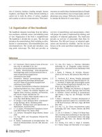
2.33 Example (functionalgraph)Considerthefunctionf : {1, 2, ,13}−→{1, 2, ,13}
defined by f (1) = 4 , f(2) = 11, f (3) = 1, f(4) = 6, f (5) = 3, f(6) = 9, f (7) = 3,
f(8) = 11, f(9) = 1, f(10) = 2, f(11) = 10, f(12) = 4, f (13) = 7. The functional
graph of f is shown in Figure 2.1. 
As Figure 2.1 illustrates, a functional graph may have several components (maximal
connected subgraphs), each component consisting of a directed cycle and some directed
trees attached to the cycle.
2.34 Fact As n tends to infinity, the following statements regarding the functional digraph of a
random function f from F
n

are true:
(i) The expected number of components is
1
2
ln n.
c
1997 by CRC Press, Inc. — See accompanying notice at front of chapter.
§
2.1 Probability theory 55
13
7
5
3
12 4
1
9
6
8
11
2
10
Figure 2.1:
A functional graph (see Example 2.33).
(ii) The expected number of points which are on the cycles is

πn/2.
(iii) The expected number of terminal points (points which have no preimages) is n/e.
(iv) The expected number of k-th iterate image points (x is a k-th iterate image point if
x = f(f(···f
  

k times
(y) ···)) for some y)is(1 −τ
k
)n,wheretheτ
k
satisfy the recurrence
τ
0
=0, τ
k+1
= e
−1+τ
k
for k ≥ 0.
2.35 Definition Let f be a random function from {1, 2, ,n} to {1, 2, ,n} and let u ∈
{1, 2, ,n}. Consider the sequence of points u
0
,u
1
,u
2
, defined by u
0
= u, u
i
=
f(u
i−1
) for i ≥ 1. In terms of the functional graph of f , this sequence describes a path that
connects to a cycle.

(i) The number of edges in the path is called the tail length of u, denoted λ(u).
(ii) The number of edges in the cycle is called the cycle length of u, denoted µ(u).
(iii) The rho-length of u is the quantity ρ(u)=λ(u)+µ(u).
(iv) The tree size of u is the number of edges in the maximal tree rooted on a cycle in the
component that contains u.
(v) The component size of u is the number of edges in the component that contains u.
(vi) The predecessors size of u is the number of iterated preimages of u.
2.36 Example The functional graph in Figure 2.1 has 2 components and 4 terminal points. The
point u =3has parameters λ(u)=1, µ(u)=4, ρ(u)=5. The tree, component, and
predecessors sizes of u =3are 4, 9,and3, respectively. 
2.37 Fact As n tends to infinity, the following are the expectations of some parameters associ-
ated with a random point in {1, 2, ,n} and a random function from F
n
: (i) tail length:

πn/8 (ii) cycle length:

πn/8 (iii) rho-length:

πn/2 (iv) tree size: n/3 (v) compo-
nent size: 2n/3 (vi) predecessors size:

πn/8.
2.38 Fact As n tends to infinity, the expectations of the maximum tail, cycle, and rho lengths in
a random functionfromF
n
are c
1
√
n, c

2
√
n,andc
3
√
n, respectively,wherec
1
≈ 0.78248,
c
2
≈ 1.73746,andc
3
≈ 2.4149.
Facts 2.37 and 2.38 indicate that in the functional graph of a random function, most
points are grouped together in one giant component, and there is a small number of large
trees. Also, almost unavoidably,a cycle of length about
√
n arises after following a path of
length
√
n edges.
Handbook of Applied Cryptography by A. Menezes, P. van Oorschot and S. Vanstone.
56 Ch. 2 Mathematical Background
2.2 Information theory
2.2.1 Entropy
Let X be a random variable which takes on a finite set of values x
1
,x
2
, ,x

n
, with prob-
ability P (X = x
i
)=p
i
,where0 ≤ p
i
≤ 1 for each i, 1 ≤ i ≤ n, and where

n
i=1
p
i
=1.
Also, let Y and Z be random variables which take on finite sets of values.
The entropy of X is a mathematical measure of the amount of information provided by
an observation of X. Equivalently,it is the uncertainity about the outcomebeforean obser-
vation of X. Entropy is also useful for approximating the average number of bits required
to encode the elements of X.
2.39 Definition The entropy or uncertainty of X is defined to be H(X)=−

n
i=1
p
i
lg p
i
=


n
i=1
p
i
lg

1
p
i

where, by convention, p
i
·lg p
i
= p
i
·lg

1
p
i

=0if p
i
=0.
2.40 Fact (properties of entropy)LetX be a random variable which takes on n values.
(i) 0 ≤ H(X) ≤ lg n.
(ii) H(X)=0if and only if p
i
=1for some i,andp

j
=0for all j = i (that is, there is
no uncertainty of the outcome).
(iii) H(X)=lgn if and only if p
i
=1/n for each i, 1 ≤ i ≤ n (that is, all outcomes are
equally likely).
2.41 Definition The joint entropy of X and Y is defined to be
H(X, Y )=−

x,y
P (X = x, Y = y)lg(P (X = x, Y = y)),
where the summation indices x and y range over all values of X and Y , respectively. The
definition can be extended to any number of random variables.
2.42 Fact If X and Y are random variables, then H(X, Y ) ≤ H(X)+H(Y ), with equality if
and only if X and Y are independent.
2.43 Definition If X, Y are random variables, the conditional entropy of X given Y = y is
H(X|Y = y)=−

x
P (X = x|Y = y)lg(P(X = x|Y = y)),
where the summation index x ranges over all values of X.Theconditional entropy of X
given Y , also called the equivocation of Y about X,is
H(X|Y )=

y
P (Y = y)H(X|Y = y),
where the summation index y ranges over all values of Y .
2.44 Fact (properties of conditional entropy)LetX and Y be random variables.
(i) The quantity H(X|Y ) measures the amount of uncertainty remaining about X after

Y has been observed.
c
1997 by CRC Press, Inc. — See accompanying notice at front of chapter.
§
2.3 Complexity theory 57
(ii) H(X|Y ) ≥ 0 and H(X|X)=0.
(iii) H(X, Y )=H(X)+H(Y |X)=H(Y )+H(X|Y ).
(iv) H(X|Y ) ≤ H(X), with equality if and only if X and Y are independent.
2.2.2 Mutual information
2.45 Definition The mutual information or transinformation of random variables X and Y is
I(X; Y )=H(X) − H(X|Y ). Similarly, the transinformation of X and the pair Y , Z is
defined to be I(X; Y,Z)=H(X) − H(X|Y,Z).
2.46 Fact (properties of mutual transinformation)
(i) The quantity I(X; Y ) can be thought of as the amount of information that Y reveals
about X. Similarly, the quantity I(X; Y, Z ) can be thought of as the amount of in-
formation that Y and Z together reveal about X.
(ii) I(X; Y ) ≥ 0.
(iii) I(X; Y )=0if and only if X and Y are independent (that is, Y contributes no in-
formation about X).
(iv) I(X; Y )=I(Y ; X).
2.47 Definition The conditional transinformation of the pair X, Y given Z is defined to be
I
Z
(X; Y )=H(X|Z) − H(X|Y,Z).
2.48 Fact (properties of conditional transinformation)
(i) The quantity I
Z
(X; Y ) can be interpreted as the amount of information that Y pro-
vides about X, given that Z has already been observed.
(ii) I(X; Y,Z )=I(X; Y )+I

Y
(X; Z).
(iii) I
Z
(X; Y )=I
Z
(Y ; X).
2.3 Complexity theory
2.3.1 Basic definitions
The maingoalof complexity theoryis to providemechanisms for classifyingcomputational
problems according to the resources needed to solve them. The classification should not
depend on a particular computational model, but rather should measure the intrinsic dif-
ficulty of the problem. The resources measured may include time, storage space, random
bits, number of processors, etc., but typically the main focus is time, and sometimes space.
2.49 Definition An algorithm is a well-defined computational procedure that takes a variable
input and halts with an output.
Handbook of Applied Cryptography by A. Menezes, P. van Oorschot and S. Vanstone.
58 Ch. 2 Mathematical Background
Of course, the term “well-definedcomputationalprocedure”is not mathematically pre-
cise. It can be made so by using formal computational models such as Turing machines,
random-access machines, or boolean circuits. Rather than get involved with the technical
intricacies of these models, it is simpler to think of an algorithm as a computer program
written in some specific programming language for a specific computer that takes a vari-
able input and halts with an output.
It is usually of interest to find the most efficient (i.e., fastest) algorithm for solving a
givencomputationalproblem. Thetime thatanalgorithmtakes tohalt dependsonthe “size”
oftheproblem instance. Also, the unitoftime usedshouldbe madeprecise, especially when
comparing the performance of two algorithms.
2.50 Definition The size of the input is the total number of bits needed to represent the input
in ordinary binary notation using an appropriate encoding scheme. Occasionally, the size

of the input will be the number of items in the input.
2.51 Example (sizes of some objects)
(i) The number of bits in the binary representation of a positive integer n is 1+lg n
bits. For simplicity, the size of n will be approximated by lg n.
(ii) If f is a polynomial of degree at most k, each coefficientbeinga non-negativeinteger
at most n, then the size of f is (k +1)lgn bits.
(iii) If A is a matrix with r rows, s columns, and with non-negative integer entries each
at most n, then the size of A is rs lg n bits. 
2.52 Definition The running time of an algorithm on a particular input is the number of prim-
itive operations or “steps” executed.
Often a step is taken to mean a bit operation. For some algorithms it will be more con-
venient to take step to mean something else such as a comparison, a machine instruction, a
machine clock cycle, a modular multiplication, etc.
2.53 Definition The worst-case running time of an algorithm is an upper bound on the running
time for any input, expressed as a function of the input size.
2.54 Definition The average-case running time of an algorithm is the average running time
over all inputs of a fixed size, expressed as a function of the input size.
2.3.2 Asymptotic notation
It is often difficult to derive the exact running time of an algorithm. In such situations one
is forced to settle for approximations of the running time, and usually may only derive the
asymptotic running time. That is, one studies how the running time of the algorithm in-
creases as the size of the input increases without bound.
In what follows, the only functions consideredare those which are defined on the posi-
tive integers and take on real values that are always positive from some point onwards. Let
f and g be two such functions.
2.55 Definition (order notation)
(i) (asymptotic upper bound) f(n)=O(g(n)) if there exists a positive constant c and a
positive integer n
0
such that 0 ≤ f(n) ≤ cg(n) for all n ≥ n

0
.
c
1997 by CRC Press, Inc. — See accompanying notice at front of chapter.
§
2.3 Complexity theory 59
(ii) (asymptotic lower bound) f(n)=Ω(g(n)) if there exists a positive constant c and a
positive integer n
0
such that 0 ≤ cg(n) ≤ f(n) for all n ≥ n
0
.
(iii) (asymptotic tight bound) f(n)=Θ(g(n)) if there exist positive constants c
1
and c
2
,
and a positive integer n
0
such that c
1
g(n) ≤ f(n) ≤ c
2
g(n) for all n ≥ n
0
.
(iv) (o-notation) f(n)=o(g(n)) if for any positive constant c>0 thereexists a constant
n
0
> 0 such that 0 ≤ f(n) <cg(n) for all n ≥ n

0
.
Intuitively, f(n)=O(g(n)) means that f grows no faster asymptotically than g(n) to
within a constant multiple, while f(n)=Ω(g(n)) means that f(n) grows at least as fast
asymptotically as g(n) to within a constant multiple. f(n)=o(g(n)) means that g(n) is an
upper bound for f(n) that is not asymptotically tight, or in other words, the function f(n)
becomes insignificant relative to g(n) as n gets larger. The expression o(1) is often used to
signify a function f(n) whose limit as n approaches ∞ is 0.
2.56 Fact (properties of order notation) For any functions f(n), g(n), h(n),andl(n),thefol-
lowing are true.
(i) f(n)=O(g(n)) if and only if g(n)=Ω(f (n)).
(ii) f(n)=Θ(g(n)) if and only if f(n)=O(g(n)) and f(n)=Ω(g(n)).
(iii) If f(n)=O(h(n)) and g(n)=O(h(n)),then(f + g)(n)=O(h(n)).
(iv) If f(n)=O(h(n)) and g(n)=O(l(n)),then(f ·g)(n)=O(h(n)l(n)).
(v) (reflexivity) f(n)=O(f(n)).
(vi) (transitivity)Iff(n)=O(g(n)) and g(n)=O(h(n)),thenf(n)=O(h(n)).
2.57 Fact (approximations of some commonly occurring functions)
(i) (polynomial function)Iff (n) is a polynomial of degree k with positive leading term,
then f(n)=Θ(n
k
).
(ii) For any constant c>0, log
c
n =Θ(lgn).
(iii) (Stirling’s formula) For all integers n ≥ 1,
√
2πn

n
e


n
≤ n! ≤
√
2πn

n
e

n+(1/(12n))
.
Thus n!=
√
2πn

n
e

n

1+Θ(
1
n
)

. Also, n!=o(n
n
) and n!=Ω(2
n
).

(iv) lg(n!) = Θ(n lg n).
2.58 Example (comparative growth rates of some functions)Let and c be arbitrary constants
with 0 <<1 <c. The following functions are listed in increasing order of their asymp-
totic growth rates:
1 < ln ln n<ln n<exp(
√
ln n ln ln n) <n

<n
c
<n
ln n
<c
n
<n
n
<c
c
n
. 
2.3.3 Complexity classes
2.59 Definition A polynomial-time algorithm is an algorithm whose worst-case running time
function is of the form O(n
k
),wheren is the input size and k is a constant. Any algorithm
whose running time cannot be so bounded is called an exponential-time algorithm.
Roughly speaking, polynomial-time algorithms can be equated with good or efficient
algorithms, while exponential-time algorithms are considered inefficient. There are, how-
ever, some practical situations when this distinction is not appropriate. When considering
polynomial-timecomplexity, the degreeofthe polynomialis significant. For example, even

Handbook of Applied Cryptography by A. Menezes, P. van Oorschot and S. Vanstone.
60 Ch. 2 Mathematical Background
though an algorithm with a running time of O(n
ln ln n
), n being the input size, is asymptot-
ically slower that an algorithm with a running time of O(n
100
), the former algorithm may
be faster in practice for smaller values of n, especially if the constants hidden by the big-O
notation are smaller. Furthermore, in cryptography, average-case complexity is more im-
portant than worst-case complexity — a necessary condition for an encryption scheme to
be considered secure is that the correspondingcryptanalysis problem is difficult on average
(or more precisely, almost always difficult), and not just for some isolated cases.
2.60 Definition A subexponential-time algorithm is an algorithm whose worst-case running
time function is of the form e
o(n)
,wheren is the input size.
A subexponential-timealgorithmis asymptoticallyfaster than an algorithmwhose run-
ning time is fully exponential in the input size, while it is asymptotically slower than a
polynomial-time algorithm.
2.61 Example (subexponential running time)LetA be an algorithm whose inputs are either
elements of a finite field F
q
(see §2.6), or an integer q. If the expected running time of A is
of the form
L
q
[α, c]=O

exp


(c + o(1))(ln q)
α
(ln ln q)
1−α

, (2.3)
where c is a positive constant, and α is a constant satisfying 0 <α<1,thenA is a
subexponential-time algorithm. Observe that for α =0, L
q
[0,c] is a polynomial in ln q,
while for α =1, L
q
[1,c] is a polynomial in q, and thus fully exponential in ln q. 
For simplicity, the theory of computational complexity restricts its attention to deci-
sion problems, i.e., problems which have either YES or NO as an answer. This is not too
restrictive in practice, as all the computational problems that will be encountered here can
be phrased as decision problems in such a way that an efficient algorithm for the decision
problem yields an efficient algorithm for the computational problem, and vice versa.
2.62 Definition The complexity class P is the set of all decision problems that are solvable in
polynomial time.
2.63 Definition The complexity class NP is the set of all decision problems for which a YES
answercanbeverifiedinpolynomialtimegivensomeextrainformation, called a certificate.
2.64 Definition The complexity class co-NP is the set of all decision problems for which a NO
answer can be verified in polynomial time using an appropriate certificate.
It must be emphasizedthat if a decision problemis in NP, it may not be the casethatthe
certificate of a YES answer can be easily obtained; what is asserted is that such a certificate
does exist, and, if known, can be used to efficiently verify the YES answer. The same is
true of the NO answers for problems in co-NP.
2.65 Example (problem in NP) Consider the following decision problem:

COMPOSITES
INSTANCE: A positive integer n.
QUESTION: Is n composite? That is, are there integers a, b > 1 such that n = ab?
COMPOSITES belongsto NP because if anintegern is composite, thenthis factcanbe
verified in polynomialtime if oneis given a divisor a of n,where1 <a<n(the certificate
in this case consists of the divisor a). It is in fact also the case that COMPOSITES belongs
to co-NP. It is still unknown whether or not COMPOSITES belongs to P. 
c
1997 by CRC Press, Inc. — See accompanying notice at front of chapter.
§
2.3 Complexity theory 61
2.66 Fact P ⊆ NP and P ⊆ co-NP.
The following are among the outstanding unresolved questions in the subject of com-
plexity theory:
1. Is P = NP?
2. Is NP = co-NP?
3. Is P = NP ∩co-NP?
Mostexpertsare oftheopinion thattheanswer toeachofthe threequestionsisNO, although
nothing along these lines has been proven.
The notion of reducibility is useful when comparing the relative difficulties of prob-
lems.
2.67 Definition Let L
1
and L
2
be two decision problems. L
1
is said to polytime reduce to L
2
,

written L
1
≤
P
L
2
, if there is an algorithm that solves L
1
which uses, as a subroutine, an
algorithm for solving L
2
, and which runs in polynomial time if the algorithm for L
2
does.
Informally, if L
1
≤
P
L
2
,thenL
2
is at least as difficult as L
1
, or, equivalently, L
1
is
no harder than L
2
.

2.68 Definition Let L
1
and L
2
be two decision problems. If L
1
≤
P
L
2
and L
2
≤
P
L
1
,then
L
1
and L
2
are said to be computationally equivalent.
2.69 Fact Let L
1
, L
2
,andL
3
be three decision problems.
(i) (transitivity)IfL

1
≤
P
L
2
and L
2
≤
P
L
3
,thenL
1
≤
P
L
3
.
(ii) If L
1
≤
P
L
2
and L
2
∈ P,thenL
1
∈ P.
2.70 Definition A decision problem L is said to be NP-complete if

(i) L ∈ NP,and
(ii) L
1
≤
P
L for every L
1
∈ NP.
The class of all NP-complete problems is denoted by NPC.
NP-complete problems are the hardest problems in NP in the sense that they are at
least as difficult as everyotherproblemin NP. There are thousandsofproblems drawn from
diverse fields such as combinatorics, number theory, and logic, that are known to be NP-
complete.
2.71 Example (subset sum problem)Thesubset sum problem is the following: given a set of
positive integers {a
1
,a
2
, ,a
n
} and a positive integer s, determine whether or not there
is a subset of the a
i
that sum to s. The subset sum problem is NP-complete. 
2.72 Fact Let L
1
and L
2
be two decision problems.
(i) If L

1
is NP-complete and L
1
∈ P,thenP = NP.
(ii) If L
1
∈ NP, L
2
is NP-complete, and L
2
≤
P
L
1
,thenL
1
is also NP-complete.
(iii) If L
1
is NP-complete and L
1
∈ co-NP,thenNP = co-NP.
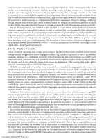
By Fact 2.72(i), if a polynomial-time algorithm is found for any single NP-complete
problem, then it is the case that P = NP, a result that would be extremely surprising. Hence,
a proof that a problem is NP-complete provides strong evidence for its intractability. Fig-
ure 2.2 illustrates what is widely believed to be the relationship between the complexity
classes P, NP, co-NP,andNPC.
Fact 2.72(ii) suggests the following procedure for proving that a decision problem L
1
is NP-complete:

Handbook of Applied Cryptography by A. Menezes, P. van Oorschot and S. Vanstone.
62 Ch. 2 Mathematical Background
co-NP
NPC
NP
P
NP ∩ co-NP
Figure 2.2:
Conjectured relationship between the complexity classes P, NP, co-NP, and NPC.
1. Prove that L
1
∈ NP.
2. Select a problem L
2
that is known to be NP-complete.
3. Prove that L
2
≤
P
L
1
.
2.73 Definition Aproblemis NP-hard if thereexists someNP-completeproblemthat polytime
reduces to it.
Note that the NP-hard classification is not restricted to only decision problems. Ob-
serve also that an NP-complete problem is also NP-hard.
2.74 Example (NP-hard problem) Given positive integers a
1
,a
2

, ,a
n
and a positive inte-
ger s, the computational version of the subset sum problem would ask to actually find a
subset of the a
i
which sums to s, provided that such a subset exists. This problem is NP-
hard. 
2.3.4 Randomized algorithms
The algorithms studied so far in this section have been deterministic; such algorithms fol-
low the same executionpath (sequence of operations) each time they execute with the same
input. By contrast, a randomized algorithm makes random decisions at certain points in
the execution; hence their execution paths may differ each time they are invoked with the
same input. The random decisions are based upon the outcome of a random number gen-
erator. Remarkably, there are many problems for which randomized algorithms are known
that are more efficient, both in terms of time and space, than the best known deterministic
algorithms.
Randomized algorithms for decision problems can be classified according to the prob-
ability that they return the correct answer.
2.75 Definition Let A be a randomized algorithm for a decision problem L,andletI denote
an arbitrary instance of L.
(i) A has 0-sided error if P (A outputs YES | I’s answer is YES )=1,and
P (A outputs YES | I’s answer is NO )=0.
(ii) A has 1-sided error if P (A outputs YES | I’s answer is YES ) ≥
1
2
,and
P (A outputs YES | I’s answer is NO )=0.
c
1997 by CRC Press, Inc. — See accompanying notice at front of chapter.

§
2.4 Number theory 63
(iii) A has 2-sided error if P (A outputs YES | I’s answer is YES ) ≥
2
3
,and
P (A outputs YES | I’s answer is NO ) ≤
1
3
.
The number
1
2
in the definition of 1-sided error is somewhat arbitrary and can be re-
placed by any positive constant. Similarly, the numbers
2
3
and
1
3
in the definition of 2-sided
error, can be replaced by
1
2
+  and
1
2
− , respectively, for any constant , 0 <<
1
2

.
2.76 Definition The expected runningtimeofarandomizedalgorithm is an upperboundonthe
expected running time for each input (the expectation being over all outputs of the random
number generator used by the algorithm), expressed as a function of the input size.
The important randomized complexity classes are defined next.
2.77 Definition (randomized complexity classes)
(i) The complexity class ZPP (“zero-sided probabilistic polynomial time”) is the set of
all decision problems for which there is a randomized algorithm with 0-sided error
which runs in expected polynomial time.
(ii) The complexity class RP (“randomized polynomial time”) is the set of all decision
problems for which there is a randomized algorithm with 1-sided error which runs in
(worst-case) polynomial time.
(iii) The complexity class BPP (“bounded error probabilistic polynomial time”) is the set
of all decision problems for which there is a randomizedalgorithmwith 2-sided error
which runs in (worst-case) polynomial time.
2.78 Fact P ⊆ ZPP ⊆ RP ⊆ BPP and RP ⊆ NP.
2.4 Number theory
2.4.1 The integers
The set of integers { ,−3, −2, −1, 0, 1, 2, 3, } is denoted by the symbol Z.
2.79 Definition Let a, b be integers. Then a divides b (equivalently: a is a divisor of b,ora is
a factor of b) if there exists an integer c such that b = ac.Ifa divides b, then this is denoted
by a|b.
2.80 Example (i) −3|18,since18 = (−3)(−6). (ii) 173|0,since0 = (173)(0). 
The following are some elementary properties of divisibility.
2.81 Fact (properties of divisibility) For all a, b, c ∈ Z, the following are true:
(i) a|a.
(ii) If a|b and b|c,thena|c.
(iii) If a|b and a|c,thena|(bx + cy) for all x, y ∈ Z.
(iv) If a|b and b|a,thena = ±b.
Handbook of Applied Cryptography by A. Menezes, P. van Oorschot and S. Vanstone.

64 Ch. 2 Mathematical Background
2.82 Definition (division algorithm for integers)Ifa and b are integers with b ≥ 1,thenor-
dinary long division of a by b yields integers q (the quotient)andr (the remainder)such
that
a = qb + r, where 0 ≤ r<b.
Moreover, q and r are unique. The remainder of the division is denoted a mod b,andthe
quotient is denoted a div b.
2.83 Fact Let a, b ∈ Z with b =0.Thena div b = a/b and a mod b = a − ba/b.
2.84 Example If a =73, b =17,thenq =4and r =5. Hence 73 mod 17 = 5 and
73 div 17 = 4. 
2.85 Definition An integer c is a common divisor of a and b if c|a and c|b.
2.86 Definition A non-negative integer d is the greatest common divisor of integers a and b,
denoted d =gcd(a, b),if
(i) d is a common divisor of a and b;and
(ii) whenever c|a and c|b,thenc|d.
Equivalently, gcd(a, b) is the largest positive integer that divides both a and b, with the ex-
ception that gcd(0, 0) = 0.
2.87 Example The commondivisorsof 12 and18 are {±1, ±2, ±3, ±6},andgcd(12, 18) = 6.

2.88 Definition A non-negative integer d is the least common multiple of integers a and b,de-
noted d =lcm(a, b),if
(i) a|d and b|d;and
(ii) whenever a|c and b|c,thend|c.
Equivalently, lcm(a, b) is the smallest non-negative integer divisible by both a and b.
2.89 Fact If a and b are positive integers, then lcm(a, b)=a · b/ gcd(a, b).
2.90 Example Since gcd(12, 18) = 6, it follows that lcm(12, 18) = 12 · 18/6=36. 
2.91 Definition Two integersa andb are said to berelativelyprime orcoprimeifgcd(a, b)=1.
2.92 Definition An integer p ≥ 2 is said to be prime if its only positive divisors are 1 and p.
Otherwise, p is called composite.
The following are some well known facts about prime numbers.

2.93 Fact If p is prime and p|ab, then either p|a or p|b (or both).
2.94 Fact There are an infinite number of prime numbers.
2.95 Fact (prime number theorem)Letπ(x) denote the number of prime numbers ≤ x.Then
lim
x→∞
π(x)
x/ ln x
=1.
c
1997 by CRC Press, Inc. — See accompanying notice at front of chapter.
§
2.4 Number theory 65
This means that for large values of x, π(x) is closely approximated by the expres-
sion x/ ln x. For instance, when x =10
10
, π(x) = 455, 052, 511, whereas x/ ln x =
434, 294, 481. A more explicit estimate for π(x) is given below.
2.96 Fact Let π(x) denote the number of primes ≤ x. Then for x ≥ 17
π(x) >
x
ln x
and for x>1
π(x) < 1.25506
x
ln x
.
2.97 Fact (fundamental theorem of arithmetic) Every integer n ≥ 2 has a factorization as a
product of prime powers:
n = p
e

1
1
p
e
2
2
···p
e
k
k
,
where the p
i
are distinct primes, and the e
i
are positive integers. Furthermore, the factor-
ization is unique up to rearrangement of factors.
2.98 Fact If a = p
e
1
1
p
e
2
2
···p
e
k
k
, b = p

f
1
1
p
f
2
2
···p
f
k
k
, where each e
i
≥ 0 and f
i
≥ 0,then
gcd(a, b)=p
min(e
1
,f
1
)
1
p
min(e
2
,f
2
)
2

···p
min(e
k
,f
k
)
k
and
lcm(a, b)=p
max(e
1
,f
1
)
1
p
max(e
2
,f
2
)
2
···p
max(e
k
,f
k
)
k
.

2.99 Example Let a = 4864 = 2
8
· 19, b = 3458 = 2 · 7 ·13 · 19.Thengcd(4864, 3458) =
2 ·19 = 38 and lcm(4864, 3458) = 2
8
·7 · 13 · 19 = 442624. 
2.100 Definition For n ≥ 1,letφ(n) denote the number of integers in the interval [1,n] which
are relatively prime to n. Thefunctionφ is called the Eulerphifunction (orthe Euler totient
function).
2.101 Fact (properties of Euler phi function)
(i) If p is a prime, then φ(p)=p − 1.
(ii) The Euler phi function is multiplicative.Thatis,ifgcd(m, n)=1,thenφ(mn)=
φ(m) ·φ(n).
(iii) If n = p
e
1
1
p
e
2
2
···p
e
k
k
is the prime factorization of n,then
φ(n)=n

1 −
1

p
1

1 −
1
p
2

···

1 −
1
p
k

.
Fact 2.102 gives an explicit lower bound for φ(n).
2.102 Fact For all integers n ≥ 5,
φ(n) >
n
6lnlnn
.
Handbook of Applied Cryptography by A. Menezes, P. van Oorschot and S. Vanstone.
66 Ch. 2 Mathematical Background
2.4.2 Algorithms in Z
Let a and b be non-negative integers, each less than or equal to n. Recall (Example 2.51)
that the number of bits in the binary representation of n is lg n +1, and this number is
approximatedby lg n. The number of bit operations for the four basic integer operations of
addition, subtraction, multiplication, and division using the classical algorithms is summa-
rized in Table 2.1. These algorithms are studied in more detail in §14.2. More sophisticated

techniques for multiplication and division have smaller complexities.
Operation Bit complexity
Addition a + b O(lg a +lgb)=O(lg n)
Subtraction a −b O(lg a +lgb)=O(lg n)
Multiplication a · b O((lg a)(lg b)) = O((lg n)
2
)
Division a = qb + r O((lg q)(lg b)) = O((lg n)
2
)
Table 2.1:
Bit complexity of basic operations in Z.
The greatest common divisor of two integers a and b can be computed via Fact 2.98.
However, computing a gcd by first obtaining prime-power factorizations does not result in
an efficient algorithm, as the problem of factoring integers appears to be relatively diffi-
cult. The Euclidean algorithm (Algorithm 2.104) is an efficient algorithm for computing
the greatest common divisor of two integers that does not require the factorization of the
integers. It is based on the following simple fact.
2.103 Fact If a and b are positive integers with a>b,thengcd(a, b)=gcd(b, a mod b).
2.104 Algorithm Euclidean algorithm for computing the greatest common divisor of two integers
INPUT: two non-negative integers a and b with a ≥ b.
OUTPUT: the greatest common divisor of a and b.
1. While b =0do the following:
1.1 Set r←a mod b, a←b, b←r.
2. Return(a).
2.105 Fact Algorithm 2.104 has a running time of O((lg n)
2
) bit operations.
2.106 Example (Euclidean algorithm) The following are the division steps of Algorithm 2.104
for computing gcd(4864, 3458) = 38:

4864 = 1 · 3458 + 1406
3458 = 2 · 1406 + 646
1406 = 2 · 646 + 114
646 = 5 · 114 + 76
114 = 1 · 76 + 38
76 = 2 ·38 + 0. 
c
1997 by CRC Press, Inc. — See accompanying notice at front of chapter.
§
2.4 Number theory 67
The Euclideanalgorithmcan be extendedso that itnotonlyyields thegreatest common
divisor d of two integers a and b, but also integers x and y satisfying ax + by = d.
2.107 Algorithm Extended Euclidean algorithm
INPUT: two non-negative integers a and b with a ≥ b.
OUTPUT: d =gcd(a, b) and integers x, y satisfying ax + by = d.
1. If b =0then set d←a, x←1, y←0, and return(d,x,y).
2. Set x
2
←1, x
1
←0, y
2
←0, y
1
←1.
3. While b>0 do the following:
3.1 q←a/b, r←a − qb, x←x
2
− qx
1

, y←y
2
− qy
1
.
3.2 a←b, b←r, x
2
←x
1
, x
1
←x, y
2
←y
1
,and y
1
←y.
4. Set d←a, x←x
2
, y←y
2
, and return(d,x,y).
2.108 Fact Algorithm 2.107 has a running time of O((lg n)
2
) bit operations.
2.109 Example (extended Euclidean algorithm) Table 2.2 shows the steps of Algorithm 2.107
with inputs a = 4864 and b = 3458. Hence gcd(4864, 3458) = 38 and (4864)(32) +
(3458)(−45) = 38. 
q r x y a b x

2
x
1
y
2
y
1
− − − − 4864 3458 1 0 0 1
1 1406 1 −1 3458 1406 0 1 1 −1
2 646 −2 3 1406 646 1 −2 −1 3
2 114 5 −7 646 114 −2 5 3 −7
5 76 −27 38 114 76 5 −27 −7 38
1 38 32 −45 76 38 −27 32 38 −45
2 0 −91 128 38 0 32 −91 −45 128
Table 2.2:
Extended Euclidean algorithm (Algorithm 2.107) with inputs a = 4864, b = 3458.
Efficient algorithms for gcd and extended gcd computations are further studied in §14.4.
2.4.3 The integers modulo n
Let n be a positive integer.
2.110 Definition If a and b are integers, then a is said to be congruent to b modulo n, written
a ≡ b (mod n),ifn divides (a−b). The integer n is called the modulusof the congruence.
2.111 Example (i) 24 ≡ 9(mod5)since 24 − 9=3·5.
(ii) −11 ≡ 17 (mod 7) since −11 − 17 = −4 · 7. 
2.112 Fact (properties of congruences) For all a, a
1
, b, b
1
, c ∈ Z, the following are true.
(i) a ≡ b (mod n) if and only if a and b leave the same remainder when divided by n.
(ii) (reflexivity) a ≡ a (mod n).

(iii) (symmetry)Ifa ≡ b (mod n) then b ≡ a (mod n).
Handbook of Applied Cryptography by A. Menezes, P. van Oorschot and S. Vanstone.
68 Ch. 2 Mathematical Background
(iv) (transitivity)Ifa ≡ b (mod n) and b ≡ c (mod n),thena ≡ c (mod n).
(v) If a ≡ a
1
(mod n) and b ≡ b
1
(mod n),thena + b ≡ a
1
+ b
1
(mod n) and
ab ≡ a
1
b
1
(mod n).
The equivalence class of an integer a is the set of all integers congruent to a modulo
n. From properties (ii), (iii), and (iv) above, it can be seen that for a fixed n the relation of
congruence modulo n partitions Z into equivalence classes. Now, if a = qn + r,where
0 ≤ r<n,thena ≡ r (mod n). Hence each integer a is congruent modulo n to a unique
integer between 0 and n −1, called the least residue of a modulo n. Thus a and r are in the
same equivalence class, and so r may simply be used to represent this equivalence class.
2.113 Definition The integers modulo n, denoted Z
n
, is the set of (equivalence classes of) in-
tegers {0, 1, 2, ,n− 1}. Addition, subtraction, and multiplication in Z
n
are performed

modulo n.
2.114 Example Z
25
= {0, 1, 2, ,24}.InZ
25
, 13 + 16 = 4,since13 + 16 = 29 ≡ 4
(mod 25). Similarly, 13 · 16 = 8 in Z
25
. 
2.115 Definition Let a ∈ Z
n
.Themultiplicative inverse of a modulo n is an integer x ∈ Z
n
such that ax ≡ 1(modn).Ifsuchanx exists, then it is unique, and a is said to be invert-
ible,oraunit; the inverse of a is denoted by a
−1
.
2.116 Definition Let a, b ∈ Z
n
. Division of a by b modulon is the product of a and b
−1
modulo
n, and is only defined if b is invertible modulo n.
2.117 Fact Let a ∈ Z
n
.Thena is invertible if and only if gcd(a, n)=1.
2.118 Example The invertible elements in Z
9
are 1, 2, 4, 5, 7,and8. For example, 4
−1

=7
because 4 ·7 ≡ 1(mod9). 
The following is a generalization of Fact 2.117.
2.119 Fact Let d =gcd(a, n). The congruence equation ax ≡ b (mod n) has a solution x if
and only if d divides b, in which case there are exactly d solutions between 0 and n − 1;
these solutions are all congruent modulo n/d.
2.120 Fact (Chinese remainder theorem, CRT) If the integers n
1
,n
2
, ,n
k
are pairwise rela-
tively prime, then the system of simultaneous congruences
x ≡ a
1
(mod n
1
)
x ≡ a
2
(mod n
2
)
.
.
.
x ≡ a
k
(mod n

k
)
has a unique solution modulo n = n
1
n
2
···n
k
.
2.121 Algorithm (Gauss’s algorithm) The solution x to the simultaneous congruences in the
Chinese remainder theorem (Fact 2.120) may be computed as x =

k
i=1
a
i
N
i
M
i
mod n,
where N
i
= n/n
i
and M
i
= N
−1
i

mod n
i
. These computations can be performed in
O((lg n)
2
) bit operations.
c
1997 by CRC Press, Inc. — See accompanying notice at front of chapter.
§
2.4 Number theory 69
Another efficient practical algorithm for solving simultaneous congruences in the Chinese
remainder theorem is presented in §14.5.
2.122 Example The pair of congruences x ≡ 3(mod7), x ≡ 7 (mod 13) has a unique solu-
tion x ≡ 59 (mod 91). 
2.123 Fact If gcd(n
1
,n
2
)=1,then thepair ofcongruencesx ≡ a (mod n
1
), x ≡ a (mod n
2
)
has a unique solution x ≡ a (mod n
1
n
2
).
2.124 Definition The multiplicative group of Z
n

is Z
∗
n
= {a ∈ Z
n
| gcd(a, n)=1}. In
particular, if n is a prime, then Z
∗
n
= {a | 1 ≤ a ≤ n −1}.
2.125 Definition The order of Z
∗
n
is defined to be the number of elements in Z
∗
n
, namely |Z
∗
n
|.
It follows from the definition of the Euler phi function (Definition 2.100) that |Z
∗
n
| =
φ(n). Note also that if a ∈ Z
∗
n
and b ∈ Z
∗
n

,thena · b ∈ Z
∗
n
,andsoZ
∗
n
is closed under
multiplication.
2.126 Fact Let n ≥ 2 be an integer.
(i) (Euler’s theorem)Ifa ∈ Z
∗
n
,thena
φ(n)
≡ 1(modn).
(ii) If n is a product ofdistinct primes, andifr ≡ s (mod φ(n)),thena
r
≡ a
s
(mod n)
for all integers a. In other words, when working modulo such an n, exponents can
be reduced modulo φ(n).
A special case of Euler’s theorem is Fermat’s (little) theorem.
2.127 Fact Let p be a prime.
(i) (Fermat’s theorem)Ifgcd(a, p)=1,thena
p−1
≡ 1(modp).
(ii) If r ≡ s (mod p − 1),thena
r
≡ a

s
(mod p) for all integers a. In other words,
when working modulo a prime p, exponents can be reduced modulo p −1.
(iii) In particular, a
p
≡ a (mod p) for all integers a.
2.128 Definition Let a ∈ Z
∗
n
.Theorder of a, denoted ord(a), is the least positive integer t such
that a
t
≡ 1(modn).
2.129 Fact If the order of a ∈ Z
∗
n
is t,anda
s
≡ 1(modn),thent divides s. In particular,
t|φ(n).
2.130 Example Let n =21.ThenZ
∗
21
= {1, 2, 4, 5, 8, 10, 11, 13, 16, 17, 19, 20}. Note that
φ(21) = φ(7)φ(3) = 12 = |Z
∗
21
|. The orders of elements in Z
∗
21

are listed in Table 2.3. 
a ∈ Z
∗
21
1 2 4 5 8 10 11 13 16 17 19 20
order of a 1 6 3 6 2 6 6 2 3 6 6 2
Table 2.3:
Orders of elements in Z
∗
21
.
2.131 Definition Let α ∈ Z
∗
n
. If the order of α is φ(n),thenα is said to be a generator or a
primitive element of Z
∗
n
.IfZ
∗
n
has a generator, then Z
∗
n
is said to be cyclic.
Handbook of Applied Cryptography by A. Menezes, P. van Oorschot and S. Vanstone.
70 Ch. 2 Mathematical Background
2.132 Fact (properties of generators of Z
∗
n

)
(i) Z
∗
n
has a generator if and only if n =2, 4,p
k
or 2p
k
,wherep is an odd prime and
k ≥ 1. In particular, if p is a prime, then Z
∗
p
has a generator.
(ii) If α is a generator of Z
∗
n
,thenZ
∗
n
= {α
i
mod n | 0 ≤ i ≤ φ(n) − 1}.
(iii) Suppose that α is a generator of Z
∗
n
.Thenb = α
i
mod n is also a generator of Z
∗
n

if and only if gcd(i, φ(n)) = 1. It follows that if Z
∗
n
is cyclic, then the number of
generators is φ(φ(n)).
(iv) α ∈ Z
∗
n
is a generator of Z
∗
n
if and only if α
φ(n)/p
≡ 1(modn) for each prime
divisor p of φ(n).
2.133 Example Z
∗
21
is not cyclic since it does not contain an element of order φ(21) = 12 (see
Table 2.3); note that 21 does not satisfy the condition of Fact 2.132(i). On the other hand,
Z
∗
25
is cyclic, and has a generator α =2. 
2.134 Definition Let a ∈ Z
∗
n
. a is said to be a quadratic residue modulo n,orasquare modulo
n, if there exists an x ∈ Z
∗

n
such that x
2
≡ a (mod n).Ifnosuchx exists, then a is called
a quadratic non-residue modulo n. The set of all quadratic residues modulo n is denoted
by Q
n
and the set of all quadratic non-residues is denoted by Q
n
.
Note that by definition 0 ∈ Z
∗
n
, whence 0 ∈ Q
n
and 0 ∈ Q
n
.
2.135 Fact Let p be an odd prime and let α be a generator of Z
∗
p
.Thena ∈ Z
∗
p
is a quadratic
residue modulo p if and only if a = α
i
mod p,wherei is an even integer. It follows that
|Q
p

| =(p −1)/2 and |Q
p
| =(p − 1)/2; that is, half of the elements in Z
∗
p
are quadratic
residues and the other half are quadratic non-residues.
2.136 Example α =6is a generator of Z
∗
13
. The powers of α are listed in the following table.
i 0 1 2 3 4 5 6 7 8 9 10 11
α
i
mod 13 1 6 10 8 9 2 12 7 3 5 4 11
Hence Q
13
= {1, 3, 4, 9, 10, 12}and Q
13
= {2, 5, 6, 7, 8, 11}. 
2.137 Fact Let n be a product of two distinct odd primes p and q, n = pq.Thena ∈ Z
∗
n
is a
quadratic residue modulo n if and only if a ∈ Q
p
and a ∈ Q
q
. It follows that |Q
n

| =
|Q
p
|·|Q
q
| =(p − 1)(q −1)/4 and |Q
n
| =3(p − 1)(q −1)/4.
2.138 Example Let n =21.ThenQ
21
= {1, 4, 16}and Q
21
= {2, 5, 8, 10, 11, 13, 17, 19, 20}.

2.139 Definition Let a ∈ Q
n
.Ifx ∈ Z
∗
n
satisfies x
2
≡ a (mod n),thenx is called a square
root of a modulo n.
2.140 Fact (number of square roots)
(i) If p is an odd prime and a ∈ Q
p
,thena has exactly two square roots modulo p.
(ii) More generally, let n = p
e
1

1
p
e
2
2
···p
e
k
k
where the p
i
are distinct odd primes and e
i
≥
1.Ifa ∈ Q
n
,thena has precisely 2
k
distinct square roots modulo n.
2.141 Example The squareroots of 12 modulo 37 are 7 and 30. The square roots of 121 modulo
315 are 11, 74, 101, 151, 164, 214, 241,and304. 
c
1997 by CRC Press, Inc. — See accompanying notice at front of chapter.
§
2.4 Number theory 71
2.4.4 Algorithms in Z
n
Let n be a positive integer. As before, the elements of Z
n
will be represented by the integers

{0, 1, 2, ,n− 1}.
Observe that if a, b ∈ Z
n
,then
(a + b)modn =

a + b, if a + b<n,
a + b −n, if a + b ≥ n.
Hence modular addition (and subtraction) can be performed without the need of a long di-
vision. Modular multiplication of a and b may be accomplished by simply multiplying a
and b as integers, and then taking the remainder of the result after division by n. Inverses
in Z
n
can be computed using the extended Euclidean algorithm as next described.
2.142 Algorithm Computing multiplicative inverses in Z
n
INPUT: a ∈ Z
n
.
OUTPUT: a
−1
mod n, provided that it exists.
1. Use the extendedEuclideanalgorithm(Algorithm2.107)to find integersx and y such
that ax + ny = d,whered =gcd(a, n).
2. If d>1,thena
−1
mod n does not exist. Otherwise, return(x).
Modular exponentiation can be performed efficiently with the repeated square-and-
multiply algorithm (Algorithm 2.143), which is crucial for many cryptographic protocols.
One version of this algorithm is based on the following observation. Let the binary repre-

sentation of k be

t
i=0
k
i
2
i
, where each k
i
∈{0, 1}.Then
a
k
=
t

i=0
a
k
i
2
i
=(a
2
0
)
k
0
(a
2

1
)
k
1
···(a
2
t
)
k
t
.
2.143 Algorithm Repeated square-and-multiply algorithm for exponentiation in Z
n
INPUT: a ∈ Z
n
, and integer 0 ≤ k<nwhose binary representation is k =

t
i=0
k
i
2
i
.
OUTPUT: a
k
mod n.
1. Set b←1.Ifk =0then return(b).
2. Set A←a.
3. If k

0
=1then set b←a.
4. For i from 1 to t do the following:
4.1 Set A←A
2
mod n.
4.2 If k
i
=1then set b←A ·b mod n.
5. Return(b).
2.144 Example (modularexponentiation)Table 2.4showsthe stepsinvolvedin thecomputation
of 5
596
mod 1234 = 1013. 
The number of bit operationsforthe basic operationsinZ
n
is summarized in Table 2.5.
Efficient algorithms for performing modular multiplication and exponentiation are further
examined in §14.3 and §14.6.
Handbook of Applied Cryptography by A. Menezes, P. van Oorschot and S. Vanstone.