Tài liệu Mạng thần kinh thường xuyên cho dự đoán P7 ppt

Recurrent Neural Networks for Prediction
Authored by Danilo P. Mandic, Jonathon A. Chambers
Copyright
c
2001 John Wiley & Sons Ltd
ISBNs: 0-471-49517-4 (Hardback); 0-470-84535-X (Electronic)
7
Stability Issues in RNN
Architectures
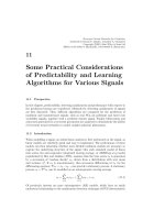
7.1 Perspective
The focus of this chapter is on stability and convergence of relaxation realised through
NARMA recurrent neural networks. Unlike other commonly used approaches, which
mostly exploit Lyapunov stability theory, the main mathematical tool employed in
this analysis is the contraction mapping theorem (CMT), together with the fixed
point iteration (FPI) technique. This enables derivation of the asymptotic stability
(AS) and global asymptotic stability (GAS) criteria for neural relaxive systems. For
rigour, existence, uniqueness, convergence and convergence rate are considered and the
analysis is provided for a range of activation functions and recurrent neural networks
architectures.
7.2 Introduction
Stability and convergence are key issues in the analysis of dynamical adaptive sys-
tems, since the analysis of the dynamics of an adaptive system can boil down to the
discovery of an attractor (a stable equilibrium) or some other kind of fixed point. In
neural associative memories, for instance, the locally stable equilibrium states (attrac-
tors) store information and form neural memory. Neural dynamics in that case can be
considered from two aspects, convergence of state variables (memory recall) and the
number, position, local stability and domains of attraction of equilibrium states (mem-
ory capacity). Conveniently, LaSalle’s invariance principle (LaSalle 1986) is used to
analyse the state convergence, whereas stability of equilibria are analysed using some
sort of linearisation (Jin and Gupta 1996). In addition, the dynamics and conver-
gence of learning algorithms for most types of neural networks may be explained and

analysed using fixed point theory.
Let us first briefly introduce some basic definitions. The full definitions and further
details are given in Appendix I. Consider the following linear, finite dimensional,
116 INTRODUCTION
autonomous system
1
of order N
y(k)=
N

i=1
a
i
(k)y(k − i)=a
T
(k)y(k − 1). (7.1)
Definition 7.2.1 (see Kailath (1980) and LaSalle (1986)). The system (7.1)
is said to be asymptotically stable in Ω ⊆ R
N
, if for any y(0), lim
k→∞
y(k)=0,for
a(k) ∈ Ω.
Definition 7.2.2 (see Kailath (1980) and LaSalle (1986)). The system (7.1) is
globally asymptotically stable if for any initial condition and any sequence a(k), the
response y(k) tends to zero asymptotically.
For NARMA systems realised via neural networks, we have
y(k +1)=Φ(y(k), w(k)). (7.2)
Let Φ(k, k
0

, Y
0
) denote the trajectory of the state change for all k  k
0
, with
Φ(k
0
,k
0
, Y
0
)=Y
0
.IfΦ(k, k
0
, Y
∗
)=Y
∗
for all k  0, then Y
∗
is called an equi-
librium point. The largest set D(Y
∗
) for which this is true is called the domain of
attraction of the equilibrium Y
∗
.IfD(Y
∗
)=R

N
and if Y
∗
is asymptotically stable,
then Y
∗
is said to be asymptotically stable in large or globally asymptotical ly stable.
It is important to clarify the difference between asymptotic stability and abso-
lute stability. Asymptotic stability may depend upon the input (initial conditions),
whereas global asymptotic stability does not depend upon initial conditions. There-
fore, for an absolutely stable neural network, the system state will converge to one
of the asymptotically stable equilibrium states regardless of the initial state and the
input signal. The equilibrium points include the isolated minima as well as the maxima
and saddle points. The maxima and saddle points are not stable equilibrium points.
Robust stability for the above discussed systems is still under investigation (Bauer et
al. 1993; Jury 1978; Mandic and Chambers 2000c; Premaratne and Mansour 1995).
In conventional nonlinear systems, the system is said to be globally asymptotically
stable, or asymptotically stable in large, if it has a unique equilibrium point which is
globally asymptotically stable in the sense of Lyapunov. In this case, for an arbitrary
initial state x(0) ∈ R
N
, the state trajectory φ(k, x(0), s) will converge to the unique
equilibrium point x
∗
, satisfying
x
∗
= lim
k→∞
φ[k, x(0), s]. (7.3)

Stability in this context has been considered in terms of Lyapunov stability and M-
matrices (Forti and Tesi 1994; Liang and Yamaguchi 1997). To apply the Lyapunov
method to a dynamical system, a neural system has to be mapped onto a new system
for which the origin is at an equilibrium point. If the network is stable, its ‘energy’ will
decrease to a minimum as the system approaches and attains its equilibrium state. If
a function that maps the objective function onto an ‘energy function’ can be found,
then the network is guaranteed to converge to its equilibrium state (Hopfield and
1
Stability of systems of this type is discussed in Appendix H.
STABILITY ISSUES IN RNN ARCHITECTURES 117
0 1 2 3 4 5 6
0
1
2
3
4
5
6
K(x)=sqrt(2x+3)
y=x
Fixed Point x
*
=3
x
K(x),y
Figure 7.1 FPI solution for roots of F (x)=x
2
− 2x − 3
Tank 1985; Luh et al. 1998). The Lyapunov stability of neural networks is studied in
detail in Han et al. (1989) and Jin and Gupta (1996).

The concept of fixed point will be central to much of what follows, for which the
basic theorems and principles are introduced in Appendix G.
Point x
∗
is called a fixed point of a function K if it satisfies K(x
∗
)=x
∗
, i.e. the
value x
∗
is unchanged under the application of function K. For instance, the roots of
function F (x)=x
2
−2x − 3 can be found by rearranging x
k+1
= K(x
k
)=
√
2x
k
+3
via fixed point iteration. The roots of the above function are −1 and 3. The FPI
which started from x
0
= 4 converges to within 10
−5
of the exact solution in nine
steps, which is depicted in Figure 7.1. This example is explained in more detail in

Appendix G.
One of the virtues of neural networks is their processing power, which rests upon
their ability to converge to a set of fixed points in the state space. Stability analysis,
therefore, is essential for the derivation of conditions that assure convergence to these
fixed points. Stability, although necessary, is not sufficient for effective processing
(see Appendix H), since in practical applications, it is desirable that a neural system
converges to only a preselected set of fixed points. In the remainder of this chapter,
two different aspects of equilibrium, i.e. the static aspect (existence and uniqueness
of equilibrium states) and the dynamic aspect (global stability, rate of convergence),
are studied. While analysing global asymptotic stability,
2
it is convenient to study the
static problem of the existence and uniqueness of the equilibrium point first, which is
the necessary condition for GAS.
2
It is important to note that the iterates of random Lipschitz functions converge if the functions
are contracting on the average (Diaconis and Freedman 1999). The theory of random operators is
a probabilistic generalisation of operator theory. The study of probabilistic operator theory and its
applications was initiated by the Prague school under the direction of Antonin Spacek, in the 1950s
(Bharucha-Reid 1976). They recognised that it is necessary to take into consideration the fact that
the operators used to describe the behaviour of systems may not be known exactly. The application
of this theory in signal processing is still under consideration and can be used to analyse stochastic
learning algorithms (Chambers et al. 2000).
118 OVERVIEW
7.3 Overview
The role of the nonlinear activation function in the global asymptotic convergence of
recurrent neural networks is studied. For a fixed input and weights, a repeated appli-
cation of the nonlinear difference equation which defines the output of a recurrent
neural network is proven to be a relaxation, provided the activation function satis-
fies the conditions required for a contraction mapping. This relaxation is shown to

exhibit linear asymptotic convergence. Nesting of modular recurrent neural networks
is demonstrated to be a fixed point iteration in a spatial form.
7.4 A Fixed Point Interpretation of Convergence in Networks with a
Sigmoid Nonlinearity
To solve many problems in the field of optimisation, neural control and signal process-
ing, dynamic neural networks need to be designed to have only a unique equilibrium
point. The equilibrium point ought to be globally stable to avoid the risk of spuri-
ous responses or the problem of local minima. Global asymptotic stability (GAS) has
been analysed in the theory of both linear and nonlinear systems (Barnett and Storey
1970; Golub and Van Loan 1996; Haykin 1996a; Kailath 1980; LaSalle 1986; Priest-
ley 1991). For nonlinear systems, it is expected that convergence in the GAS sense
depends not only on the values of the parameter vector, but also on the parameters
of the nonlinear function involved. As systems based upon sigmoid functions exhibit
stability in the bounded input bounded output (BIBO) sense, due to the saturation
type sigmoid nonlinearity, we investigate the characteristics of the nonlinear activa-
tion function to obtain GAS for a general RNN-based nonlinear system. In that case,
both the external input vector to the system x(k) and the parameter vector w(k) are
assumed to be a time-invariant part of the system under fixed point iteration.
7.4.1 Some Properties of the Logistic Function
To derive the conditions which the nonlinear activation function of a neuron should
satisfy to enable convergence of real-time learning algorithms, activation functions
of a neuron are analysed in the framework of contraction mappings and fixed point
iteration.
Observation 7.4.1. The logistic function
Φ(x)=
1
1+e
−βx
(7.4)
is a contraction on [a, b] ∈ R for 0 <β<4 and the iteration

x
i+1
= Φ(x
i
) (7.5)
converges to a unique solution x
∗
from ∀x
0
∈ [a, b] ∈ R.
Proof. By the contraction mapping theorem (CMT) (Appendix G), function K is a
contraction on [a, b] ∈ R if
STABILITY ISSUES IN RNN ARCHITECTURES 119
abK(a) K(b)
Figure 7.2 The contraction mapping
(i) x ∈ [a, b] ⇒ K(x) ∈ [a, b],
(ii) ∃γ<1 ∈ R
+
s.t. |K(x) − K(y)|  γ|x − y|∀x, y ∈ [a, b].
The condition (i) is illustrated in Figure 7.2. The logistic function (7.4) is strictly
monotonically increasing, since its first derivative is strictly greater than zero. Hence,
in order to prove that Φ is a contraction on [a, b] ∈ R, it is sufficient to prove that it
contracts the upper and lower bound of interval [a, b], i.e. a and b, which in turn gives
• a − Φ(a)  0,
• b − Φ(b)  0.
These conditions will be satisfied if the function Φ is smaller in magnitude than the
curve y = x, i.e. if
|x| >





1
1+e
−βx




,β>0. (7.6)
Condition (ii) can be proven using the mean value theorem (MVT) (Luenberger 1969).
Namely, as the logistic function Φ (7.4) is differentiable, for ∀x, y ∈ [a, b], ∃ξ ∈ (a, b)
such that
|Φ(x) − Φ(y)| = |Φ

(ξ)(x − y)| = |Φ

(ξ)||x − y|. (7.7)
The first derivative of the logistic function (7.4) is
Φ

(x)=

1
1+e
−βx


=
βe

−βx
(1+e
−βx
)
2
, (7.8)
which is strictly positive, and for which the maximum value is Φ

(0) = β/4. Hence,
for β  4, the first derivative Φ

 1. Finally, for γ<1 ⇔ β<4, function Φ given
in (7.4) is a contraction on [a, b] ∈ R .
Convergence of FPI: if x
∗
is a zero of x − Φ(x) = 0, or in other words the fixed
point of function Φ, then for γ<1(β<4)
|x
i
− x
∗
| = |Φ(x
i−1
) − Φ(x
∗
)|  γ|x
i−1
− x
∗
|. (7.9)

Thus, since for γ<1 ⇒{γ}
i
i
−→ 0
|x
i
− x
∗
|  γ
i
|x
0
− x
∗
|⇒ lim
i→∞
x
i
= x
∗
(7.10)
and iteration x
i+1
= Φ(x
i
) converges to some x
∗
∈ [a, b].
Convergence/divergence of the FPI clearly depends on the size of slope β in Φ.
Considering the general nonlinear system Equation (7.2), this means that for a fixed

input vector to the iterative process and fixed weights of the network, an FPI solution
depends on the slope (first derivative) of the nonlinear activation function and some
measure of the weight vector. If the solution exists, that is the only value to which
120 CONVERGENCE IN NETWORKS WITH A SIGMOID NONLINEARITY
−10 −5 0 5 10
0
0.1
0.2
0.3
0.4
0.5
0.6
0.7
0.8
0.9
1
x
Φ(x)
(a) The logistic nonlinear function
−10 −5 0 5 10
0
0.05
0.1
0.15
0.2
0.25
x
Φ
′
(x)

(b) The first derivative of the logistic
function
Figure 7.3 The logistic function and its derivative
−5 0 5
−1
−0.8
−0.6
−0.4
−0.2
0
0.2
0.4
0.6
0.8
1
y=x
x
Φ(x)
β=1
β=0.25
β=8
(a) Centred logistic functions
−5 0 5
−0.5
0
0.5
1
1.5
y=x
x

Φ(x)
β=1
β=0.25
β=8
(b) Unipolar logistic functions
Figure 7.4 Various logistic functions
such a relaxation algorithm converges. Figure 7.3 shows the logistic function and its
first derivative for β = 1. To depict Observation 7.4.1 further, we use a centred logistic
function (Φ−mean(Φ)), as shown in Figure 7.4(a). For Φ a contraction, the condition
(i) from CMT (Appendix G) must be satisfied. That is the case if the values of Φ are
smaller in magnitude than the corresponding values of the function y = x. As shown
in Figure 7.4(a), that condition is satisfied for a range of logistic functions with the
slope 0 <β<4. Indeed, e.g. for β = 8, the logistic function has an intersection
with the function y = x (dotted curve in Figure 7.4(a)), which means that for β>4,
there are regions in Φ where (a −Φ(a))  0, which violates condition (i) of CMT and
Observation 7.4.1.
STABILITY ISSUES IN RNN ARCHITECTURES 121
7.4.2 Logistic Function, Rate of Convergence and Fixed Point Theory
The rate of convergence of a fixed point iteration can be judged by the closeness of
x
k+1
to x
∗
relative to the closeness of x
k
to x
∗
(Dennis and Schnabel 1983; Gill et al.
1981).
Definition 7.4.2. A sequence {x

k
} is said to converge towards its fixed point x
∗
with order r if
0  lim
k→∞
x
k+1
− x
∗

x
k
− x
∗

r
< ∞, (7.11)
where r ∈ N is the largest number such that the above inequality holds.
Since we are interested in the value of r that occurs in the limit, r is sometimes
called the asymptotic convergence rate.Ifr = 1, the sequence is said to exhibit linear
convergence, if r = 2, the sequence is said to exhibit quadratic convergence.
Definition 7.4.3. For a sequence {x
k
} which has an order of convergence r, the
asymptotic error constant of the fixed point iteration is the value γ ∈ R
+
which
satisfies
γ = lim

k→∞
x
k+1
− x
∗

x
k
− x
∗

r
. (7.12)
When r = 1, i.e. for linear convergence, γ must be strictly less than unity in order
for convergence to occur (Gill et al. 1981).
Example 7.4.4. Show that the convergent FPI process
x
i+1
= Φ(x
i
) (7.13)
exhibits a linear asymptotic convergence for which the error constant equals |Φ

(x
∗
)|.
Solution. Consider the ratio |e
i+1
|/|e
i

| of successive errors, where e
i
= x
i
− x
∗
|e
i+1
|
|e
i
|
=
|x
i+1
− x
∗
|
|x
i
− x
∗
|
=
|Φ(x
i
) − Φ(x
∗
)|
|x

i
− x
∗
|
MVT
= |Φ

(ξ)| (7.14)
for some ξ ∈ (x
i
,x
∗
). Having in mind that the iteration (7.13) converges to x
∗
when
i →∞
lim
i→∞
|e
i+1
|
|e
i
|
= lim
i→∞
|Φ

(ξ)| = |Φ


(x
∗
)|. (7.15)
Therefore, iteration (7.13) exhibits linear asymptotic convergence with convergence
rate |Φ

(x
∗
)|.
Example 7.4.5. Derive the error bound e
i
= |x
i
− x
∗
| for the FPI process
x
i+1
= Φ(x
i
). (7.16)
Solution. Rewrite the error bound as
x
i
− x
∗
= Φ(x
i−1
) − Φ(x
i

)+Φ(x
i
) − Φ(x
∗
) (7.17)
and therefore
|x
i
− x
∗
|  γ|x
i−1
− x
i
| + γ|x
i
− x
∗
|. (7.18)
122 CONVERGENCE IN NETWORKS WITH A SIGMOID NONLINEARITY
Table 7.1 Fixed point iterates for the logistic function
Starting value x
0
−10 10
First iterate 0.000 045 1
Second iterate 0.5 0.7311
Third iterate 0.6225 0.6750
Fourth iterate 0.6508 0.6626
Fifth iterate 0.6572 0.6598
Sixth iterate 0.6586 0.6592

Seventh iterate 0.6589 0.6591
1 2 3 4 5 6 7 8
−10
−8
−6
−4
−2
0
2
4
6
8
10
Number of iteration
Iterates
Initial value x
0
=−10
Initial value x
0
=10
Figure 7.5 FPI for a logistic function and different initial values
Hence
|x
i
− x
∗
| 
γ
1 − γ

|x
i−1
− x
i
|. (7.19)
Example 7.4.6. Show that when repeatedly applying logistic function Φ the interval
[−10, 10] degenerates towards a point ζ ∈ [−10, 10].
Solution. Observation 7.4.1 provides a general background for this example. Notice
that β = 1. In order to show that a function converges in the FPI sense, it is sufficient
to show that it contracts the bound points of the interval [−10, 10], since it is a strictly
monotonically increasing function. Let us therefore set up the iteration
x
i+1
= Φ(x
i
),x
0
∈{−10, 10}. (7.20)
STABILITY ISSUES IN RNN ARCHITECTURES 123
0 0.5 1 1.5 2 2.5 3 3.5 4 4.5 5
0.5
0.55
0.6
0.65
0.7
0.75
0.8
0.85
0.9
0.95

1
slope of nonlinearity
fixed point
Figure 7.6 Fixed points for the logistic nonlinearity, as a function of slope β and starting
point x
0
=10
The results of the iteration are given in Table 7.1 and Figure 7.5. As seen from
Table 7.1, for both initial values, function Φ provides a contraction of the underlying
interval, i.e. it provides a set of mappings
Φ :[−10, 10] → [0.000 045, 1],
Φ :[0.000 045, 1] → [0.5, 0.7311],
.
.
.
Φ : ζ → ζ.











(7.21)
Indeed, the iterates from either starting point x
0

∈{−10, 10} converge to a value
ζ ∈ [0.6589, 0.6591] ∈ [−10, 10]. It can be shown that after 24 iterations, the fixed
point ζ is
Φ :[−10, 10]
i
−→ ζ =0.659 046 068 407 41, (7.22)
which is shown in Figure 7.5.
Example 7.4.7. Plot the fixed points of the logistic function
Φ(x)=
1
1+e
−βx
(7.23)
for a range of β.
Solution. The result of the experiment is shown in Figure 7.6. From Figure 7.6, the
values of the fixed point increase with β and converge to unity when β increases.
Example 7.4.8. Show that the logistic function from Example 7.4.6, exhibits a linear
asymptotic convergence for which the convergence rate is γ =0.2247.
124 CONVERGENCE OF NONLINEAR RELAXATION
Table 7.2 Error convergence for the FPI of the logistic function
x
0
= −10 e
i
e
i
/e
i−1
x
0

=10 e
i
e
i
/e
i−1
First iterate 0.000 045 0.659 — 1 0.341 —
Second iterate 0.5 0.159 0.2413 0.7311 0.0721 0.2114
Third iterate 0.6225 0.0365 0.2296 0.6750 0.016 0.2219
Fourth iterate 0.6508 0.0082 0.2247 0.6626 0.0036 0.2246
Fifth iterate 0.6572 0.0018 0.2247 0.6598 0.0008 0.2247
Sixth iterate 0.6586 0.0004 0.2247 0.6592 0.0002 0.2247
Seventh iterate 0.6589 0.0001 0.2247 0.6591 0.0001 0.2247
Solution. To show that the rate of convergence of the iterative process (7.13) is
|Φ

(x
∗
)|, let us calculate Φ

(x
∗
) ≈ Φ

(0.659) = 0.2247. Let us now upgrade Table 7.1
in order to show the rate of convergence. The results are shown in Table 7.2. As
Φ

(x
∗

) ≈ 0.2247, it is expected that, according to CMT, the ratio of successive errors
converges to Φ

(x
∗
). Indeed, for either initial value in the FPI, the errors e
i
= x
i
−x
∗
decrease with the order of iteration and the ratio of successive errors e
i+1
/e
i
converges
to 0.2247 and reaches that value after as few iterations as i = 4 for x
0
= −10 and
i = 5 for x
0
= 10.
Properties of the tanh activation function in this context are given in Krcmar et
al. (2000).
Remark 7.4.9. The function
tanh(βx)=
e
βx
− e
−βx

e
βx
+e
−βx
provides contraction mapping for 0 <β<1.
This is easy to show, following the analysis for the logistic function and noting that
tanh

(βx)=4β/(e
−βx
+e
βx
)
2
, which is strictly positive and for which the maximum
value is β = 1 for x = 0. Convergence of FPI for β = 1 and β =1.2 for a tanh
activation function is shown in Figure 7.7. The graphs show convergence from two
different starting values, y = −10 and y = 10. For β = 1, relaxations from both
starting values converge towards zero, whereas for β =1.2, which is greater than the
bound given in Remark 7.4.9, we have two different fixed points. For convergence of
learning algorithms for adaptive filters based upon neural networks, we desire only
one stable fixed point, and the further emphasis will be on bounds on the weights and
nonlinearity which preserve this condition.
7.5 Convergence of Nonlinear Relaxation Equations Realised Through a
Recurrent Perceptron
We next analyse convergence towards an equilibrium based upon a recurrent percep-
tron using contraction mapping and corresponding fixed point iteration. Unlike in
the linear case, the external input data to (7.2) do not need to be a zero vector, but
simply kept constant.
STABILITY ISSUES IN RNN ARCHITECTURES 125

0 20 40 60 80 100 120 140 160 180 200
−1
−0.8
−0.6
−0.4
−0.2
0
0.2
0.4
0.6
0.8
1
y
0
=−10, β=1
y
0
=10, β=1
y
0
=10, β=1.2
y
0
=−10, β=1.2
Iteration number
Output of FPI for tanh
Figure 7.7 Fixed points for the tanh activation function
Proposition 7.5.1 (see Mandic and Chambers 1999b). GAS relaxation for a
recurrent perceptron given by
y(k +1)=Φ(u(k)

T
w(k)), (7.24)
where u
T
k
=[y(k−1), ,y(k−N), 1,x(k−1), ,x(k−M)], is a contraction mapping
and converges to some value y
∗
∈ (0, 1) for β

N
j=1
|w
j
(k)| < 4.
Proof. Equation (7.24) can be written as
y(k +1)=Φ

N+M+1

j=1
w
j
z
j
(k)

, (7.25)
where z
j

(k)isthejth element of input u(k). The iteration (7.25) is biased and can
be expressed as
y(k +1)=Φ(y(k), ,y(k − N +1), const.). (7.26)
The existence, uniqueness and convergence features of mapping (7.24), follow from
properties of the logistic function. Iteration (7.24), for a contractive Φ converges to a
fixed point y
∗
= Φ(y
∗
+ const.), where the constant is given by
const. =

N+M+1

j=N+1
w
j
z
j
(k)

.
It is assumed that the weights are not time-variant. Since the condition for convergence
of the logistic function to a fixed point is 0 <β<4, it follows that the slope in
the logistic function β and the weights w
1
, ,w
N
in the weight vector w are not
126 CONVERGENCE OF NONLINEAR RELAXATION

Table 7.3 Fixed point iterates for the NARMA perceptron
Starting value y
0
−10 10
First iterate 0.006 68 0.795 71
Second iterate 0.445 10 0.520 35
Third iterate 0.487 69 0.494 82
Fourth iterate 0.491 73 0.492 41
Fifth iterate 0.492 11 0.492 18
Sixth iterate 0.492 15 0.492 16
independent and that the effective slope in the logistic function now becomes the
product β

N
j=1
w
j
. Therefore




β
N

j=1
w
j





 β
N

j=1
|w
j
| < 4 ⇔w
1
<
4
β
(7.27)
is the condition of GAS convergence of (7.2) realised through a recurrent NARMA
perceptron.
A comparison of the nonlinear GAS result (7.27) with its linear counterpart shows
that they are both based upon the ·
1
norm of the corresponding coefficient vector.
In the nonlinear case, however, the measure of nonlinearity is also included.
Example 7.5.2. Show that the iteration
y(k)=Φ(y(k − 1)) =
1
1+e
−0.25y(k−1)+0.5
(7.28)
with initial values y
0
= −10 and y

0
= 10 converges towards a point y
∗
∈ [−10, 10].
Solution. Note that β =0.25 and w = 1. The numerical values for iteration (7.28)
are given in Table 7.3. Indeed, the iterates from either starting point converge to a
value y
∗
∈ [0.492 15, 0.492 16] ⊂ [−10, 10]. It can be shown that after 15 iterations
for y
0
= −10 and 16 iterations for y
0
= 10, the fixed point to which the FPI (7.28)
converges is y
∗
=0.492 159 969 021 68.
Corollary 7.5.3 (see Mandic and Chambers 1999b). In the case of the real-
isation of (7.2) by a NARMA recurrent perceptron, convergence towards a point in
the FPI sense does not depend on the number of external input signals, nor on their
values, as long as they are finite.
The convergence rate is the ratio of the distances between the current and previous
iterate of an FPI and a fixed point y
∗
, i.e. (y(k) − y
∗
)/(y(k − 1) − y
∗
). This reveals
how quickly an FPI process converges towards a point.

Observation 7.5.4 (see Mandic and Chambers 1999b). A realisation of an
iterative process (7.2) by a recurrent perceptron converges towards a fixed point y
∗
exhibiting linear convergence with convergence rate Φ

(y
∗
) (Example 7.4.8).
STABILITY ISSUES IN RNN ARCHITECTURES 127
0 0.5 1 1.5 2 2.5 3 3.5 4 4.5 5
0.1
0.2
0.3
0.4
0.5
0.6
0.7
0.8
0.9
1
slope of nonlinearity
fixed point
Xo=10
Xo=−10
Figure 7.8 Fixed points for the biased logistic nonlinearity
Example 7.5.5. Plot the fixed points of the biased logistic function
Φ(x)=
1
1+e
−βx+bias

(7.29)
for a range of β and bias = 2.
Solution. To depict the effects of varying β, noise was added to the system. From
Figure 7.8, the values of fixed points increase with β and converge to unity when
β increases. However, for β large enough, the fixed points to which the iteration
x
i+1
= Φ(x
i
) converges might not be unique. Indeed, the broken line in Figure 7.8
represents the iteration whose starting value was x
0
= 10, while the solid line in
Figure 7.8 represents the case with x
0
= −10. For a range of β around β = 4, the
iterations from different starting points do not converge to the same value. The values
of fixed points for the biased logistic function differ from the corresponding values for
the pure logistic function. Moreover, the fixed points differ for various values of the
bias in the biased logistic function.
Remark 7.5.6. For stability of FPI for a tanh activation function replace the bound
β<4byβ<1, i.e. w
1
< 1/β.
7.6 Relaxation in Nonlinear Systems Realised by an RNN
Let Y
i
=[y
i
1

, ,y
i
N
]
T
be a vector comprising the outputs of a general RNN
at iteration i of the FPI. The input vector to a network is u
i
=[y
i
1
, ,y
i
N
,
1,x
N+1
, ,x
N+M+1
]
T
. The weight matrix W consists of N rows and N + M +1
columns. Then, by a CMT in R
N
, the iterative process applied on the general RNN
converges, if M =[a, b]
N
is a closed subset of R
N
such that

128 RELAXATION IN NONLINEAR SYSTEMS REALISED BY AN RNN
(i) Φ : M → M;
(ii) if for some norm ·, ∃γ<1 such that Φ(x)−Φ(y)  γx −y, ∀x, y ∈ M
the equation
x = Φ(x) (7.30)
has a unique solution x
∗
∈ M , and the iteration
x
i+1
= Φ(x
i
) (7.31)
converges to x
∗
for any starting value x
0
∈ M .
Actually, since the function Φ in this case is a multivariate function, Φ =
[Φ
1
, ,Φ
N
]
T
, where N is the number of neurons of the RNN, we have a set of
mappings
y
i
1

= Φ
1
(u
T
i−1
W
1
),
.
.
.
.
.
.
y
i
N
= Φ
N
(u
T
i−1
W
N
),








(7.32)
where {W
i
} are the appropriate columns in W . An obvious problem is that the
convergence is norm dependent. Therefore, that condition should be replaced by some
condition based upon the features of Φ.
Let us denote the Jacobian of Φ by J.IfM ∈ R
N
is a convex set and Φ is
continuously differentiable on M =[a, b]
N
⊂ R
N
and satisfies the conditions of the
CMT, then
max
z∈M
J(z)  γ. (7.33)
For convergence, the FPI at every neuron should be convergent. The following analysis
gives the bound for the elements of the weight matrix W of the RNN with respect
to the derivatives of the components of Φ =[Φ
1
, ,Φ
N
]. Recall that for the case of
a single recurrent perceptron, the condition for GAS was
N


j=1
|w
j
| <
4
β
⇔w
1
<
4
β
=
1
Φ

max
.
However, for a network of N neurons, it is possible to have a convergent FPI, even if
some of the neurons violate the previous conditions. When it comes to the monotonic
convergence, it is important that the process at every neuron converges uniformly.
This is straightforward to show, since for any x, y ∈ R
N
, which are processed by a
neural network, we have
|Φ(x) − Φ(y)| =
N

i=1





N

j=1
w
i,j
Φ
j
(x
j
) −
N

j=1
w
i,j
Φ
j
(y
j
)





N

i=1

N

j=1
|w
i,j
||Φ
j
(x
j
) − Φ
j
(y
j
)|

N

j=1
|Φ

max
||x
j
− y
j
|
N

i=1
|w

i,j
|. (7.34)
STABILITY ISSUES IN RNN ARCHITECTURES 129
1 2 3 4 5 6 7 8
0.1
0.2
0.3
0.4
0.5
0.6
0.7
0.8
0.9
1
Number of iteration
Outputs of neurons
y
1
y
2
y
3
Figure 7.9 FPI for a general RNN
For uniform convergence at every particular neuron, it is the diagonal weights of the
weight matrix (self-feedback) which together with the slope β
i
have an influence on
the convergence in the FPI sense. As in the case of a recurrent NARMA perceptron,
the feedback of a general RNN may consist of a number n of delayed versions of its
output, in addition to the state feedback from the remaining neurons in the network.

In that case, the number of feedback inputs to the network becomes N + n − 1 and
the condition for GAS becomes
max
1kN
{|w
k,k
|, |w
k,N+1
|, ,|w
k,N+n−1
|} <
4
(N + n −1) max
1iN
β
i
. (7.35)
Observation 7.6.1. The rate of convergence of relaxation in RNNs does not depend
on the length of the tap delay input line.
Proof. It is already shown that all the variables related to the MA part of the under-
lying NARMA process form a constant during the FPI iteration, while the feedback
variables are updated in every iteration. Hence, no matter how many external input
signals, their contribution to the FPI relaxation is embodied in a constant. Therefore,
the iteration
Y
i+1
= Φ(Y
i
, X, W ) (7.36)
does not depend on the number of external input samples.

Example 7.6.2. Analyse the convergence of the iteration process for a general RNN
with three neurons and six external input signals and a logistic activation function.
Solution. Let us choose the initial values X
0
= rand(10, 1)∗1, W = rand(10, 3)∗2−1,
using the notation of MATLAB, and start the iteration process. Here rand(M,N)
130 THE ITERATIVE APPROACH AND NESTING
-1
No
k+1 k
y
i=1
i
i=i+1
i>m
y
i
W
X
z
(a) Iterative process
module 1 module 2 module m
yyy
WX WX W X

1
2
m
(b) Iterative process realised spatially
Figure 7.10 Spatial realisation of an iterative process

denotes an (M × N)-dimensional matrix of uniformly distributed random numbers
∈ [0, 1]. The convergence of the outputs of neurons in the FPI sense is depicted in
Figure 7.9. For every neuron, the iteration process converges or, if in vector form, the
output vector of the RNN converges to a fixed vector of the iteration.
7.7 The Iterative Approach and Nesting
Nesting corresponds to the procedure of reducing the interval size in set theory. In
signal processing, however, nesting is essentially a nonlinear spatial structure which
corresponds to the cascaded structure in linear signal processing (Baltersee and Cham-
bers 1998; Haykin and Li 1995; Mandic and Chambers 1998b; Mandic et al. 1998).
The RNN-based nested sigmoid scheme can be written as (Haykin 1994; Poggio and
Girosi 1990)
F (W, X)=Φ


n
w
n
Φ


i
v
i
Φ

···Φ


j
u

j
X
j

···

, (7.37)
where Φ is a sigmoidal function. This corresponds to a multilayer network of units
that sum their inputs with ‘weights’ W = {w
n
,v
i
, ,u
j
, } and then perform a
sigmoidal transformation of this sum. Our aim is to show that nesting can exhibit
contraction mapping and that repeatedly applied nesting can lead to convergence
in the FPI sense. Therefore, instead of having a spatial, nested, pipelined structure,
nesting can be obtained through a temporal, iterative, relaxive structure (Mandic and
Chambers 2000c), as shown in Figure 7.10. Quantities that change under iteration in
Figure 7.10 have a bar above the symbol.
STABILITY ISSUES IN RNN ARCHITECTURES 131
Observation 7.7.1. The compound nested logistic functions
ˆx = Φ(x
N
)
= Φ(Φ(x
N−1
))
.

.
.
= Φ

Φ(Φ(···(Φ(x
1
)) ···))

 
N

(7.38)
provide a contraction mapping for β<4 and the FPI converges towards a point
x
∗
∈ [a, b].
Proof. Notice that the nesting process (7.38) represents an implicitly written fixed
point iteration process
x
i+1
= Φ(x
i
) ⇔ x
i+1
= Φ(Φ(x
i−1
)) = Φ

Φ(Φ(···(Φ(x
1

)) ···))

 
N

. (7.39)
Hence, nesting (7.38) and fixed point iteration (7.13) are a realisation of the same
process and have already been considered. Let us therefore just show the diagram of
the effects of the nesting process for the logistic function with slope β = 1, depicted in
Figure 7.11. From Figure 7.11, it is apparent that nesting (7.38) provides contraction
mapping of its argument. Hence, it is expected that the nesting process (7.38) with
N stages converges towards the point x
∗
∈ [|Φ

(x
∗
)|
N
a, |Φ

(x
∗
)|
N
b]. For N small, the
fixed point iteration achieved through a nesting process (7.38) may not reach its fixed
point. However, from Tables 7.1 and 7.2 and Figure 7.11, even with N = 4, the error
|x
4

− x
∗
| < 0.01, which suffices for practical applications.
To summarise:
• for the nesting process to be a contraction mapping, the range of slopes β for
the logistic function Φ should be bounded, with 0 <β<4;
• the nesting process of a sufficient order applied to an interval [a, b] ∈ R converges
to a point x
∗
∈ [a, b], which is a fixed point of the fixed point iteration x
i+1
=
Φ(x
i
);
• the nesting process (7.38) exhibits a linear asymptotic convergence whose rate
is |Φ

(x
∗
)|, where x
∗
is the fixed point of mapping Φ.
The nesting process (7.38) provides the iteration spatially, rather than temporally.
Such a strategy is known as pipelining and is widely used in advanced computer
architectures (Hwang and Briggs 1986). Using the pipelining strategy, a task is divided
in subtasks, each of them being represented by a module. Pipelining corresponds to
unfolding the finite iterative process into a spatial structure of the same length as
the number of iterations in the former. Now, from (7.37), the pipelined structure
represents indeed a spatial realisation of an essentially temporal iterative process, and

converges under the same conditions as the nesting process (7.38). A realisation of
132 THE ITERATIVE APPROACH AND NESTING
−10 −5 0 5 10
0
0.2
0.4
0.6
0.8
1
argument
first nonlinear pass
−10 −5 0 5 10
0.5
0.55
0.6
0.65
0.7
0.75
argument
second nonlinear pass
−10 −5 0 5 10
0.62
0.63
0.64
0.65
0.66
0.67
0.68
argument
third nonlinear pass

−10 −5 0 5 10
0.65
0.655
0.66
0.665
argument
fourth nonlinear pass
Figure 7.11 Nested logistic nonlinearity
y
out
weight matrix W
module M module (M-1) module 1
weight matrix W weight matrix W
z
z
-1
-1
I
zz z
zz
-1
-1-1
-1-1
I
I
I
II
y
M
y

(M-1),1 ,12
y
,1
,1
p
ppp
(N-1) (N-1) (N-1)
M
y (k-1)
s(k-M) s(k-M+1) s(k-M+2)
(k) (k) (k)
(k)
s(k-1) s(k)
Figure 7.12 Pipelined Recurrent Neural Network
process (7.38) is the so-called pipelined recurrent neural network (PRNN) (Haykin and
Li 1995), shown in Figure 7.12, which provides a spatial form of the iteration (7.37).
Therefore, for instance, instead of having a temporal FPI on a recurrent perceptron
(Figure 6.2), it suffices, for a finite-length FPI, to consider a spatial PRNN structure.
STABILITY ISSUES IN RNN ARCHITECTURES 133
7.8 Upper Bounds for GAS Relaxation within FCRNNs
Neural systems of the form
x(k +1)=Ax(k)+Bσ[Wx(k)+s] (7.40)
have been widely considered (Jin et al. 1994). Here, x is the state vector of the network
and σ( ·) is a vector of nonlinear activation functions. On the other hand, the weight
matrix W of a recurrent neural network can be split up into the feedback part (index
a) and the feedforward part (index b), which gives Y (k +1) = Φ(W
a
Y (k)+W
b
x(k)),

which can degenerate into the form (7.40). Namely, for a contractive activation func-
tion Φ, we have (Mandic and Chambers 2000e)
Φ(a + b) <Φ(a)+Φ(b) <a+ Φ(b), (7.41)
and results for system (7.40) provide the upper bound for stability of the fully con-
nected RNN system described above (Mandic et al. 2000).
7.9 Summary
The relationships between the number of neurons in the RNN, the slope in the activa-
tion function β and a measure of W have been provided, which guarantee convergence
of a relaxation process realised by fully connected recurrent neural networks. Based
upon the fixed point iteration (FPI), it has been shown that these conditions rest
entirely upon the slope of the activation function β and a measure of the ·
1
norm
of the weight vector of a recurrent perceptron. A connection between nesting and
FPI, which is the basis of the GAS convergence, has been established, and a pipelined
recurrent neural network (PRNN) has been shown to be a spatial realisation of the
FPI process. The results obtained can be applied when recurrent neural networks are
used as computational models, in particular, as optimisation models. The results can
also be used as stability analysis tools for some classes of nonlinear control systems.