Mạng thần kinh thường xuyên cho dự đoán P12

Recurrent Neural Networks for Prediction
Authored by Danilo P. Mandic, Jonathon A. Chambers
Copyright
c
2001 John Wiley & Sons Ltd
ISBNs: 0-471-49517-4 (Hardback); 0-470-84535-X (Electronic)
12
Exploiting Inherent
Relationships Between
Parameters in Recurrent
Neural Networks
12.1 Perspective
Optimisation of complex neural network parameters is a rather involved task. It
becomes particularly difficult for large-scale networks, such as modular networks, and
for networks with complex interconnections, such as feedback networks. Therefore, if
an inherent relationship between some of the free parameters of a neural network can
be found, which holds at every time instant for a dynamical network, it would help
to reduce the number of degrees of freedom in the optimisation task of learning in a
particular network.
We derive such relationships between the gain β in the nonlinear activation function
of a neuron Φ and the learning rate η of the underlying learning algorithm for both
the gradient descent and extended Kalman filter trained recurrent neural networks.
The analysis is then extended in the same spirit for modular neural networks.
Both the networks with parallel modules and networks with nested (serial) modules
are analysed. A detailed analysis is provided for the latter, since the former can be
considered a linear combination of modules that consist of feedforward or recurrent
neural networks.
For all these cases, the static and dynamic equivalence between an arbitrary neural
network described by β, η and W (k) and a referent network described by β
R
=1,

η
R
and W
R
(k) are derived. A deterministic relationship between these parameters is
provided, which allows one degree of freedom less in the nonlinear optimisation task
of learning in this framework. This is particularly significant for large-scale networks
of any type.
12.2 Introduction
When using neural networks, many of their parameters are chosen empirically. Apart
from the choice of topology, architecture and interconnection, the parameters that
200 INTRODUCTION
influence training time and performance of a neural network are the learning rate η,
gain of the activation function β and set of initial weights W
0
. The optimal values
for these parameters are not known a priori and generally they depend on external
quantities, such as the training data. Other parameters that are also important in
this context are
• steepness of the sigmoidal activation function, defined by γβ; and
• dimensionality of the input signal to the network and dimensionality and char-
acter of the feedback for recurrent networks.
It has been shown (Thimm and Fiesler 1997a,b) that the distribution of the initial
weights has almost no influence on the training time or the generalisation performance
of a trained neural network. Hence, we concentrate on the relationship between the
parameters of a learning algorithm (η) and those of a nonlinear activation function (β).
To improve performance of a gradient descent trained network, Jacobs (1988) pro-
posed that the acceleration of convergence of learning in neural networks be achieved
through the learning rate adaptation. His arguments were that
1. every adjustable learning parameter of the cost function should have its own

learning rate parameter; and
2. every learning rate parameter should vary from one iteration to the next.
These arguments are intuitively sound. However, if there is a dependence between
some of the parameters in the network, this approach would lead to suboptimal learn-
ing and oscillations, since coupled parameters would be trained using different learning
rates and different speed of learning, which would deteriorate the performance of the
network. To circumvent this problem, some heuristics on the values of the parameters
have been derived (Haykin 1994). To shed further light onto this problem and offer
feasible solutions, we therefore concentrate on finding relationships between coupled
parameters in recurrent neural networks. The derived relationships are also valid for
feedforward networks, since recurrent networks degenerate into feedforward networks
when the feedback is removed.
Let us consider again a common choice for the activation function,
Φ(γ,β,x)=
γ
1+e
−βx
. (12.1)
This is a Φ : R → (0,γ) function. The parameter β is called the gain and the product
γβ the steepness (slope) of the activation function.
1
The reciprocal of gain is also
referred to as the temperature. The gain γ of a node in a neural network is a constant
that amplifies or attenuates the net input to the node. In Kruschke and Movellan
(1991), it has been shown that the use of gradient descent to adjust the gain of the
node increases learning speed.
Let us consider again the general gradient-descent-based weight adaptation algo-
rithm, given by
W (k)=W (k − 1) − η∇
W

E(k), (12.2)
1
The gain and steepness are identical for activation functions with γ = 1. Hence, for such networks,
we often use the term slope for β.
RELATIONSHIPS BETWEEN PARAMETERS IN RNNs 201
where E(k)=
1
2
e
2
(k) is a cost function, W (k) is the weight vector/matrix at the
time-instant k and η is a learning rate. The gradient ∇
W
E(k) in (12.2) comprises
the first derivative of the nonlinear activation function (12.1), which is a function of
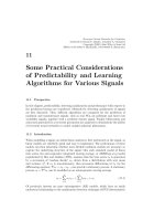
β (Narendra and Parthasarathy 1990). For instance, for a simple nonlinear FIR filter
shown in Figure 12.1, the weight update is given by
w(k +1)=w(k)+ηΦ

(x
T
(k)w(k))e(k)x(k). (12.3)
For a function Φ(β, x)=Φ(βx), which is the case for the logistic, tanh and arctan
nonlinear functions,
2
Equation (12.3) becomes
w(k +1)=w(k)+ηβΦ

(x
T

(k)w(k))e(k)x(k). (12.4)
From (12.4), if β increases, so too will the step on the error performance surface for a
fixed η. It seems, therefore, advisable to keep β constant, say at unity, and to control
the features of the learning process by adjusting the learning rate η, thereby having one
degree of freedom less, when all of the parameters in the network are adjustable. Such
reduction may be very significant for nonlinear optimisation algorithms employed for
parameter adaptation in a particular recurrent neural network.
A fairly general gradient algorithm that continuously adjusts parameters η, β and
γ can be expressed by
y(k)=Φ(X(k), W (k)),
e(k)=s(k) − y(k),
W (k +1)=W (k) −
η(k)
2
∂e
2
(k)
∂W (k)
,
η(k +1)=η(k) −
ρ
2
∂e
2
(k)
∂η(k)
,
β(k +1)=β(k) −
θ
2

∂e
2
(k)
∂β(k)
,
γ(k +1)=γ(k) −
ζ
2
∂e
2
(k)
∂γ(k)
,






































(12.5)
where ρ is a small positive constant that controls the adaptive behaviour of the step
size sequence η(k), whereas small positive constants θ and ζ control the adaptation
2
For the logistic function
σ(β, x)=
1
1+e
−βx
= σ(βx),

its first derivative becomes
dσ(β, x)
dx
= −
βe
−βx
(1 + e
−βx
)
2
,
whereas for the tanh function
tanh(β, x)=
e
βx
− e
−βx
e
βx
+e
−βx
= tanh(βx),
we have
d tanh(βx)
dx
= β
d tanh(βx)
dβx
.
The same principle is valid for the Gaussian and inverse tangent activation functions.

202 INTRODUCTION
x(k)
ww w w
12 3 N
y(k)
zzz z
-1 -1 -1 -1
(k) (k)
(k)
(k)
x(k-N+1)
Φ
x(k-1) x(k-2)
Figure 12.1 A simple nonlinear adaptive filter
of the gain of the activation function β and gain of the node γ, respectively. We will
concentrate only on adaptation of β and η.
The selection of learning rate η is critical for the gradient descent algorithms (Math-
ews and Xie 1993). An η that is small as compared to the reciprocal of the input signal
power will ensure small misadjustment in the steady state, but the algorithm will con-
verge slowly. A relatively large η, on the other hand, will provide faster convergence at
the cost of worse misadjustment and steady-state characteristics. Therefore, an ideal
choice would be an adjustable η which would be relatively large in the beginning of
adaptation and become gradually smaller when approaching the global minimum of
the error performance surface (optimal values of weights).
We illustrate the above ideas on the example of a simple nonlinear FIR filter, shown
in Figure 12.1, for which the output is given by
y(k)=Φ(x
T
(k)w(k)). (12.6)
We can continually adapt the step size using a gradient descent algorithm so as to

reduce the squared estimation error at each time instant. Extending the approach
from Mathews and Xie (1993) to the nonlinear case, we obtain
e(k)=s(k) − Φ(x
T
(k)w(k)),
w(k)=w(k − 1) + η(k − 1)e(k − 1)Φ

(k − 1)x(k − 1),
η(k)=η(k − 1) −
ρ
2
∂
∂η(k − 1)
e
2
(k)
= η(k − 1) −
ρ
2
∂
T
e
2
(k)
∂w(k)
∂w(k)
∂η(k − 1)
= η(k − 1) + ρe(k)e(k − 1)Φ

(k)Φ


(k − 1)x
T
(k − 1)x(k),























(12.7)
where Φ


(k)=Φ

(x
T
(k)w(k)), Φ

(k − 1) = Φ

(x
T
(k − 1)w(k − 1)) and ρ is a small
positive constant that controls the adaptive behaviour of the step size sequence η(k).
If we adapt the step size for each weight individually, we have
η
i
(k)=η
i
(k−1)+ρe(k)e(k−1)Φ

(k)Φ

(k−1)x
i
(k)x
i
(k−1),i=1,...,N, (12.8)
and
w
i
(k +1)=w

i
(k)+η
i
(k)e(k)x
i
(k),i=1,...,N. (12.9)
These expressions become much more complicated for large and recurrent networks.
As an alternative to the continual learning rate adaptation, we might consider
continual adaptation of the gain of the activation function Φ(βx). The gradient descent
RELATIONSHIPS BETWEEN PARAMETERS IN RNNs 203
algorithm that would update the adaptive gain can be expressed as
e(k)=s(k) − Φ(w
T
(k)x(k)),
w(k)=w(k − 1) + η(k − 1)e(k − 1)Φ

(k − 1)x(k − 1),
β(k)=β(k − 1) −
θ
2
∂
∂β(k − 1)
e
2
(k)
= β(k − 1) −
θ
2
∂
T

e
2
(k)
∂w(k)
∂w(k)
∂β(k − 1)
= β(k − 1) + θη(k − 1)e(k)e(k − 1)Φ

(k)Φ

β
(k − 1)x
T
(k − 1)x(k).
























(12.10)
For the adaptation of β(k) there is a need to calculate the second derivative of the
activation function, which is rather computationally involved. Such an adaptive gain
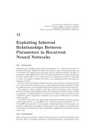
algorithm was, for instance, analysed in Birkett and Goubran (1997). The proposed
function was
σ(x, a)=





x, |x|  a,
sgn(x)

(1 − a) tanh

|x|−a
1 − a

+ a

, |x| >a,
(12.11)

where x is the input signal and a defines the adaptive linear region of the sigmoid.
This activation function is shown in Figure 12.2. Parameter a is updated according
to the stochastic gradient rule. The benefit of this algorithm is that the slope and
region of linearity of the activation function can be adjusted. Although this and
similar approaches are an alternative to the learning rate adaptation, researchers have
not taken into account that parameters β and η might be coupled. If a relationship
between them can be derived, then we choose adaptation of the parameter that is
less computationally expensive to adapt and less sensitive to adaptation errors. As
shown above, adaptation of the gain β is far more computationally expensive that
adaptation of η. Hence, there is a need to mathematically express the dependence
between the two and reduce the computational load for training neural networks.
Thimm et al. (1996) provided the relationship between the gain β of the logistic
activation function,
Φ(β,x)=
1
1+e
−βx
, (12.12)
and the learning rate η for a class of general feedforward neural networks trained
by backpropagation. They prove that changing the gain of the activation function is
equivalent to simultaneously changing the learning rate and the weights. This simpli-
fies the backpropagation learning rule by eliminating one of its parameters (Thimm
et al. 1996). This concept has been successfully applied to compensate for the non-
standard gain of optical sigmoids for optical neural networks. Relationships between
η and β for recurrent and modular networks were derived by Mandic and Chambers
(1999a,e).
Basic modular architectures are the parallel and serial architecture. Parallel archi-
tectures provide linear combinations of neural network modules, and learning algo-
rithms for them are based upon minimising the linear combination of the output
204 OVERVIEW

−5 −4 −3 −2 −1 0 1 2 3 4 5
−1
−0.8
−0.6
−0.4
−0.2
0
0.2
0.4
0.6
0.8
1
x
The adaptive sigmoid
a=0
a=0.5
a=1
Figure 12.2 An adaptive sigmoid
errors of particular modules. Hence, the algorithms for training such networks are
extensions of standard algorithms designed for single modules. Serial (nested) modu-
lar architectures are more complicated, an example of which is a pipelined recurrent
neural network (PRNN). This is an emerging architecture used in nonlinear time
series prediction (Haykin and Li 1995; Mandic and Chambers 1999f). It consists of a
number of nested small-scale recurrent neural networks as its modules, which means
that a learning algorithm for such a complex network has to perform a nonlinear
optimisation task on a number of parameters. We look at relationships between the
learning rate and the gain of the activation function for this architecture and for
various learning algorithms.
12.3 Overview
A relationship between the learning rate η in the learning algorithm and the gain β

in the nonlinear activation function, for a class of recurrent neural networks (RNNs)
trained by the real-time recurrent learning (RTRL) algorithm is provided. It is shown
that an arbitrary RNN can be obtained via the referent RNN, with some deterministic
rules imposed on its weights and the learning rate. Such relationships reduce the
number of degrees of freedom when solving the nonlinear optimisation task of finding
the optimal RNN parameters. This analysis is further extended for modular neural
architectures.
We define the conditions of static and dynamic equivalence between a referent net-
work, with β = 1, and an arbitrary network with an arbitrary β. Since the dynamic
equivalence is dependent on the chosen learning algorithm, the relationships are pro-
vided for a variety of both the gradient descent (GD) and the extended recursive
RELATIONSHIPS BETWEEN PARAMETERS IN RNNs 205
least-squares (ERLS) classes of learning algorithms and a general nonlinear activa-
tion function of a neuron.
By continuity, the derived results are also valid for feedforward networks and their
linear and nonlinear combinations.
12.4 Static and Dynamic Equivalence of Two Topologically Identical
RNNs
As the aim is to eliminate either the gain β or the learning rate η from the paradigm of
optimisation of the RNN parameters, it is necessary to derive the relationship between
a network with arbitrarily chosen parameters β and η and the referent network, so as
the outputs of the networks are identical for every time instant. An obvious choice for
the referent network is the network with the gain of the activation function β = 1. Let
us therefore denote all the entries in the referent network, which are different from
those of an arbitrary network, with the superscript ‘R’ joined to a particular variable,
i.e. β
R
=1.
For two networks to be equivalent, it is necessary that their outputs are identical
and that this is valid for both the trained network and while on the run, i.e. while

tracking some dynamical process. We therefore differentiate between the equivalence
in the static and dynamic sense. We define the static and dynamic equivalence between
two networks below.
Definition 12.4.1. By static equivalence, we consider the equivalence of the outputs
of an arbitrary network and the referent network with fixed weights, for a given input
vector u(k), at a fixed time instant k.
Definition 12.4.2. By dynamic equivalence, we consider the equivalence of the out-
puts between an arbitrary network and the referent network for a given input vector
u(k), with respect to the learning algorithm, while the networks are running.
The static equivalence is considered for already trained networks, whereas both
static and dynamic equivalence are considered for networks being adapted on the
run. We can think of the static equivalence as an analogue to the forward pass in
computation of the outputs of a neural network, whereas the dynamic equivalence
can be thought of in terms of backward pass, i.e. weight update process. We next
derive the conditions for either case.
12.4.1 Static Equivalence of Two Isomorphic RNNs
In order to establish the static equivalence between an arbitrary and referent RNN,
the outputs of their neurons must be the same, i.e.
y
n
(k)=y
R
n
(k) ⇔ Φ(u
T
n
(k)w
n
(k)) = Φ
R

(u
T
n
(k)w
R
n
(k)), (12.13)
where the index ‘n’ runs over all neurons in an RNN, and w
n
(k) and u
n
(k) are,
respectively, the set of weights and the set of inputs which belong to the neuron n.
For a general nonlinear activation function, we have
Φ(β,w
n
, u
n
)=Φ(1, w
R
n
, u
n
) ⇔ βw
n
= w
R
n
. (12.14)
206 STATIC AND DYNAMIC EQUIVALENCE OF TWO RNNs

To illustrate this, consider, for instance, the logistic nonlinearity, given by
1
1+e
−βu
T
n
w
n
=
1
1+e
−u
T
n
w
R
n
⇔ βw
n
= w
R
n
, (12.15)
where the time index (k) is neglected, since all the vectors above are constant during
the calculation of the output values. As the equality (12.14) should be valid for every
neuron in the RNN, it is therefore valid for the complete weight matrix W of the
RNN.
The essence of the above analysis is given in the following lemma, which is inde-
pendent of the underlying learning algorithm for the RNN, which makes it valid for
two isomorphic

3
RNNs of any topology and architecture.
Lemma 12.4.3 (see Mandic and Chambers 1999e). For a recurrent neural
network, with weight matrix W and gain of the activation function β, to be equivalent
in the static sense to the referent network, characterised by W
R
and β
R
=1, with
the same topology and architecture (isomorphic), the following condition must be
satisfied:
βW (k)=W
R
(k). (12.16)
12.4.2 Dynamic Equivalence of Two Isomorphic RNNs
The equivalence of two RNNs, includes both the static equivalence and dynamic
equivalence. As in the learning process (12.2), the learning rate η is multiplied by the
gradient of the cost function, we shall investigate the role of β in the gradient of the
cost function for the RNN. We are interested in a general class of nonlinear activation
functions where
∂Φ(β,x)
∂x
=
∂Φ(βx)
∂(βx)
∂(βx)
∂x
= β
∂Φ(βx)
∂(βx)

= β
∂Φ(1,x)
∂x
. (12.17)
In our case, it becomes
Φ

(β,w, u)=βΦ

(1, w
R
, u). (12.18)
Indeed, for a simple logistic function (12.12), we have
Φ

(x)=
βe
−βx
(1+e
−βx
)
2
= βΦ

(x
R
),
where x
R
= βx denotes the argument of the referent logistic function (with β

R
= 1),
so that the network considered is equivalent in the static sense to the referent net-
work. The results (12.17) and (12.18) mean that wherever Φ

occurs in the dynamical
equation of the RTRL-based learning process, the first derivative (or gradient when
applied to all the elements of the weight matrix W ) of the referent function equivalent
in the static sense to the one considered, becomes multiplied by the gain β.
The following theorem provides both the static and dynamic interchangeability of
the gain in the activation function β and the learning rate η for the RNNs trained by
the RTRL algorithm.
3
Isomorphic networks have identical topology, architecture and interconnections.