Tài liệu Lọc Kalman - lý thuyết và thực hành bằng cách sử dụng MATLAB (P2) ppt
Bạn đang xem bản rút gọn của tài liệu. Xem và tải ngay bản đầy đủ của tài liệu tại đây (217.04 KB, 31 trang )
2
Linear Dynamic Systems
What we experience of nature is in models, and all of nature's models are so beautiful.
1
R. Buckminster Fuller (1895±1983)
2.1 CHAPTER FOCUS
Models for Dynamic Systems. Since their introduction by Isaac Newton in the
seventeenth century, differential equations have provided concise mathematical
models for many dynamic systems of importance to humans. By this device,
Newton was able to model the motions of the planets in our solar system with a
small number of variables and parameters. Given a ®nite number of initial conditions
(the initial positions and velocities of the sun and planets will do) and these
equations, one can uniquely determine the positions and velocities of the planets
for all time. The ®nite-dimensional representation of a problem (in this example, the
problem of predicting the future course of the planets) is the basis for the so-called
state-space approach to the representation of differential equations and their
solutions, which is the focus of this chapter. The dependent variables of the
differential equations become state variables of the dynamic system. They explicitly
represent all the important characteristics of the dynamic system at any time.
The whole of dynamic system theory is a subject of considerably more scope than
one needs for the present undertaking (Kalman ®ltering). This chapter will stick to just
those concepts that are essential for that purpose, which is the development of the state-
space representation for dynamic systems described by systems of linear differential
equations. These are given a somewhat heuristic treatment, without the mathematical
rigor often accorded the subject, omitting the development and use of the transform
methods of functional analysis for solving differential equations when they serve no
purpose in the derivation of the Kalman ®lter. The interested reader will ®nd a more
formal and thorough presentation in most upper-level and graduate-level textbooks on
1
From an interview quoted by Calvin Tomkins in ``From in the outlaw area,'' The New Yorker, January 8,
1966.
25
Kalman Filtering: Theory and Practice Using MATLAB, Second Edition,
Mohinder S. Grewal, Angus P. Andrews
Copyright # 2001 John Wiley & Sons, Inc.
ISBNs: 0-471-39254-5 (Hardback); 0-471-26638-8 (Electronic)
ordinary differential equations. The objective of the more engineering-oriented
treatments of dynamic systems is usually to solve the controls problem, which is the
problem of de®ning the inputs (i.e., control settings) that will bring the state of the
dynamic system to a desirable condition. That is not the objective here, however.
2.1.1 Main Points to Be Covered
The objective in this chapter is to characterize the measurable outputs of dynamic
systems as functions of the internal states and inputs of the system. (The italicized
terms will be de®ned more precisely further along.) The treatment here is determi-
nistic, in order to de®ne functional relationships between inputs and outputs. In the
next chapter, the inputs are allowed to be nondeterministic (i.e., random), and the
objective of the following chapter will be to estimate the states of the dynamic
system in this context.
Dynamic Systems and Differential Equations. In the context of Kalman
®ltering, a dynamic system has come to be synonymous with a system of ordinary
differential equations describing the evolution over time of the state of a physical
system. This mathematical model is used to derive its solution, which speci®es the
functional dependence of the state variables on their initial values and the system
inputs. This solution de®nes the functional dependence of the measurable outputs on
the inputs and the coef®cients of the model.
Mathematical Models for Continuous and Discrete Time. The principal
dynamic system models are summarized in Table 2.1.
2
For implementation in digital
computers, the problem representation is transformed from an analog model (func-
tions of continuous time) to a digital model (functions de®ned at discrete times).
Observability characterizes the feasibility of uniquely determining the state of a
given dynamic system if its outputs are known. This characteristic of a dynamic
system is determinable from the parameters of its mathematical model.
2.2 DYNAMIC SYSTEMS
2.2.1 Dynamic Systems Represented by Differential Equations
A system is an assemblage of interrelated entities that can be considered as a whole.
If the attributes of interest of a system are changing with time, then it is called a
dynamic system.Aprocess is the evolution over time of a dynamic system.
Our solar system, consisting of the sun and its planets, is a physical example of a
dynamic system. The motions of these bodies are governed by laws of motion that
depend only upon their current relative positions and velocities. Sir Isaac Newton
(1642±1727) discovered these laws and expressed them as a system of differential equa-
tionsÐanother of his discoveries. From the time of Newton, engineers and scientists
have learned to de®ne dynamic systems in terms of the differential equations that
govern their behavior. They have also learned how to solve many of these differential
equations to obtain formulas for predicting the future behavior of dynamic systems.
2
These include nonlinear models, which are discussed in Chapter 5. The primary interest in this chapter
will be in linear models.
26 LINEAR DYNAMIC SYSTEMS
EXAMPLE 2.1 (below, left): Newton's Model for a Dynamic System of n
Massive Bodies For a planetary system with n bodies (idealized as point
masses), the acceleration of the ith body in any inertial (i.e., non-rotating and
non-accelerating) Cartesian coordinate system is given by Newton's third law as the
second-order differential equation
d
2
r
i
dt
2
C
g
P
n
j1
jTi
m
j
r
j
À r
i
jr
j
À r
i
j
3
; 1 i n;
where r
j
is the position coordinate vector of the jth body, m
j
is the mass of the jth
body, and C
g
is the gravitational constant. This set of n differential equations, plus
the associated initial conditions of the bodies (i.e., their initial positions and
velocities) theoretically determines the future history of the planetary system.
EXAMPLE 2.2 (above, right): The Harmonic Resonator with Linear
Damping Consider the accompanying diagram of an idealized apparatus with a
mass m attached through a spring to an immovable base and its frictional contact to
its support base represented by a dashpot. Let d be the displacement of the mass
from its position at rest, dd=dt be the velocity of the mass, and atd
2
d=dt
2
its
acceleration. The force F acting on the mass can be represented by Newton's second
law as
Ftmat
m
d
2
d
dt
2
t
Àk
s
dtÀk
d
dd
dt
t;
TABLE 2.1 Mathematical Models of Dynamic Systems
Continuous Discrete
Time invariant
Linear
_
xtFxtCut x
k
Fx
kÀ1
Gu
kÀ1
General
_
xtf xt; ut x
k
fx
kÀ1
; u
kÀ1
Time varying
Linear
_
xtF txtCtut x
k
F
kÀ1
x
kÀ1
G
kÀ1
u
kÀ1
General
_
xtf t; xt; ut x
k
fk; x
kÀ1
; u
kÀ1
0
r
4
r
3
r
1
m
1
r
2
m
2
m
3
m
4
Example 2.1 Example 2.2
2.2 DYNAMIC SYSTEMS 27
where k
s
is the spring constant and k
d
is the drag coef®cient of the dashpot. This
relationship can be written as a differential equation
m
d
2
d
dt
2
Àk
s
d À k
d
dd
dt
in which time (t) is the differential variable and displacement (d) is the dependent
variable. This equation constrains the dynamical behavior of the damped harmonic
resonator. The order of a differential equation is the order of the highest derivative,
which is 2 in this example. This one is called a linear differential equation, because
both sides of the equation are linear combinations of d and its derivatives. (That of
Example 2.1 is a nonlinear differential equation.)
Not All Dynamic Systems Can Be Modeled by Differential Equations.
There are other types of dynamic systems, such as those modeled by Petri nets or
inference nets. However, the only types of dynamic systems considered in this book
will be modeled by differential equations or by discrete-time linear state dynamic
equations derived from linear differential or difference equations.
2.2.2 State Variables and State Equations
The second-order differential equation of the previous example can be transformed
to a system of two ®rst-order differential equations in the two dependent variables
x
1
d and x
2
dd=dt. In this way, one can reduce the form of any system of higher
order differential equations to an equivalent system of ®rst-order differential
equations. These systems are generally classi®ed into the types shown in Table
2.1, with the most general type being a time-varying differential equation for
representing a dynamic system with time-varying dynamic characteristics. This is
represented in vector form as
_
xtf t; xt; ut; 2:1
where Newton's ``dot'' notation is used as a shorthand for the derivative with respect
to time, and a vector-valued function f to represent a system of n equations
_
x
1
f
1
t; x
1
; x
2
; x
3
; ; x
n
; u
1
; u
2
; u
3
; ; u
r
; t;
_
x
2
f
2
t; x
1
; x
2
; x
3
; ; x
n
; u
1
; u
2
; u
3
; ; u
r
; t;
_
x
3
f
3
t; x
1
; x
2
; x
3
; ; x
n
; u
1
; u
2
; u
3
; ; u
r
; t;
.
.
.
_
x
n
f
n
t; x
1
; x
2
; x
3
; ; x
n
; u
1
; u
2
; u
3
; ; u
r
; t
2:2
in the independent variable t (time), n dependent variables fx
i
j1 i ng, and r
known inputs fu
i
j1 i rg. These are called the state equations of the dynamic
system.
28 LINEAR DYNAMIC SYSTEMS
State Variables Represent the Degrees of Freedom of Dynamic
Systems. The variables x
1
; ; x
n
are called the state variables of the dynamic
system de®ned by Equation 2.2. They are collected into a single n-vector
xtx
1
t x
2
t x
3
t ÁÁÁ x
n
t
T
2:3
called the state vector of the dynamic system. The n-dimensional domain of the state
vector is called the state space of the dynamic system. Subject to certain continuity
conditions on the functions f
i
and u
i
; the values x
i
t
0
at some initial time t
0
will
uniquely determine the values of the solutions x
i
t on some closed time interval
t Pt
0
; t
f
with initial time t
0
and ®nal time t
f
[57]. In that sense, the initial value of
each state variable represents an independent degree of freedom of the dynamic
system. The n values x
1
t
0
; x
2
t
0
; x
3
t
0
; ; x
n
t
0
can be varied independently, and
they uniquely determine the state of the dynamic system over the time interval
t Pt
0
; t
f
.
EXAMPLE 2.3: State Space Model of the Harmonic Resonator For the
second-order differential equation introduced in Example 2.2, let the state variables
x
1
d and x
2
_
d. The ®rst state variable represents the displacement of the mass
from static equilibrium, and the second state variable represents the instantaneous
velocity of the mass. The system of ®rst-order differential equations for this dynamic
system can be expressed in matrix form as
d
dt
x
1
t
x
2
t
F
c
x
1
t
x
2
t
;
F
c
01
À
k
s
m
À
k
d
m
"#
;
where F
c
is called the coef®cient matrix of the system of ®rst-order linear differential
equations. This is an example of what is called the companion form for higher order
linear differential equations expressed as a system of ®rst-order differential equa-
tions.
2.2.3 Continuous Time and Discrete Time
The dynamic system de®ned by Equation 2.2 is an example of a continuous system,
so called because it is de®ned with respect to an independent variable t that varies
continuously over some real interval t Pt
0
; t
f
. For many practical problems,
however, one is only interested in knowing the state of a system at a discrete set
of times t Pft
1
; t
2
; t
3
; g. These discrete times may, for example, correspond to the
times at which the outputs of a system are sampled (such as the times at which Piazzi
recorded the direction to Ceres). For problems of this type, it is convenient to order
the times t
k
according to their integer subscripts:
t
0
< t
1
< t
2
< ÁÁÁt
kÀ1
< t
k
< t
k1
< ÁÁÁ:
2.2 DYNAMIC SYSTEMS 29
That is, the time sequence is ordered according to the subscripts, and the subscripts
take on all successive values in some range of integers. For problems of this type, it
suf®ces to de®ne the state of the dynamic system as a recursive relation,
xt
k1
f xt
k
; t
k
; t
k1
; 2:4
by means of which the state is represented as a function of its previous state. This is
a de®nition of a discrete dynamic system. For systems with uniform time intervals Dt
t
k
kDt:
Shorthand Notation for Discrete-Time Systems. It uses up a lot of ink if
one writes xt
k
when all one cares about is the sequence of values of the state
variable x. It is more ef®cient to shorten this to x
k
, so long as it is understood that it
stands for xt
k
, and not the kth component of x. If one must talk about a particular
component at a particular time, one can always resort to writing x
i
t
k
to remove any
ambiguity. Otherwise, let us drop t as a symbol whenever it is clear from the context
that we are talking about discrete-time systems.
2.2.4 Time-Varying Systems and Time-Invariant Systems
The term ``physical plant'' or ``plant'' is sometimes used in place of ``dynamic
system,'' especially for applications in manufacturing. In many such applications, the
dynamic system under consideration is literally a physical plantÐa ®xed facility
used in the manufacture of materials. Although the input ut may be a function of
time, the functional dependence of the state dynamics on u and x does not depend
upon time. Such systems are called time invariant or autonomous. Their solutions
are generally easier to obtain than those of time-varying systems.
2.3 CONTINUOUS LINEAR SYSTEMS AND THEIR SOLUTIONS
2.3.1 Input±Output Models of Linear Dynamic Systems
The block diagram in Figure 2.1 represents a linear continuous system with three
types of variables:
Inputs, which are under our control, and therefore known to us, or at least
measurable by us. (In the next chapter, however, they will be assumed to be
known only statistically. That is, individual samples of u are random but with
known statistical properties.)
State variables, which were described in the previous section. In most
applications, these are ``hidden variables,'' in the sense that they cannot
generally be measured directly but must be somehow inferred from what can
be measured.
Outputs, which are those things that can be known through measurements.
These concepts are discussed in greater detail in the following subsections.
30 LINEAR DYNAMIC SYSTEMS
2.3.2 Dynamic Coef®cient Matrices and Input Coupling Matrices
The dynamics of linear systems are represented by a set of n ®rst-order linear
differential equations expressible in vector form as
_
xt
d
dt
xt
FtxtCtut; 2:5
where the elements and components of the matrices and vectors can be functions of
time:
Ft
f
11
t f
12
t f
13
t ÁÁÁ f
1n
t
f
21
t f
22
t f
23
t ÁÁÁ f
2n
t
f
31
t f
32
t f
33
t ÁÁÁ f
3n
t
.
.
.
.
.
.
.
.
.
.
.
.
.
.
.
f
n1
t f
n2
t f
n3
t ÁÁÁ f
nn
t
2
6
6
6
6
6
6
6
4
3
7
7
7
7
7
7
7
5
;
Ct
c
11
t c
12
t c
13
t ÁÁÁ c
1r
t
c
21
t c
22
t c
23
t ÁÁÁ c
2r
t
c
31
t c
32
t c
33
t ÁÁÁ c
3r
t
.
.
.
.
.
.
.
.
.
.
.
.
.
.
.
c
n1
t c
n2
t c
n3
t ÁÁÁ c
nr
t
2
6
6
6
6
6
6
6
4
3
7
7
7
7
7
7
7
5
;
utu
1
t u
2
t u
3
t ÁÁÁ u
r
t
T
:
The matrix Ft is called the dynamic coef®cient matrix, or simply the dynamic
matrix. Its elements are called the dynamic coef®cients. The matrix Ct is called the
input coupling matrix, and its elements are called input coupling coef®cients. The
r-vector u is called the input vector.
Fig. 2.1 Block diagram of a linear dynamic system.
2.3 CONTINUOUS LINEAR SYSTEMS AND THEIR SOLUTIONS 31
EXAMPLE 2.4: Dynamic Equation for a Heating/Cooling System Consider
the temperature T in a heated enclosed room or building as the state variable of a
dynamic system. A simpli®ed plant model for this dynamic system is the linear
equation
_
TtÀk
c
TtÀT
o
t k
h
ut;
where the constant ``cooling coef®cient'' k
c
depends on the quality of thermal
insulation from the outside, T
o
is the temperature outside, k
h
is the heating=cooling
rate coef®cient of the heater or cooler, and u is an input function that is either u 0
(off) or u 1 (on) and can be de®ned as a function of any measurable quantities.
The outside temperature T
o
, on the other hand, is an example of an input function
which may be directly measurable at any time but is not predictable in the future. It is
effectively a random process.
2.3.3 Companion Form for Higher Order Derivatives
In general, the nth-order linear differential equation
d
n
yt
dt
n
f
1
t
d
nÀ1
yt
dt
nÀ1
ÁÁÁf
nÀ1
t
dyt
dt
f
n
tytut2:6
can be rewritten as a system of n ®rst-order differential equations. Although the state
variable representation as a ®rst-order system is not unique [56], there is a unique
way of representing it called the companion form.
Companion Form of the State Vector. For the nth-order linear dynamic
system shown above, the companion form of the state vector is
xt yt;
d
dt
yt;
d
2
dt
2
yt; ;
d
nÀ1
dt
nÀ1
yt
T
: 2:7
Companion Form of the Differential Equation. The nth-order linear differ-
ential equation can be rewritten in terms of the above state vector xt as the vector
differential equation
d
dt
x
1
t
x
2
t
.
.
.
x
nÀ1
t
x
n
t
2
6
6
6
6
6
4
3
7
7
7
7
7
5
01 0ÁÁÁ 0
00 1ÁÁÁ 0
.
.
.
.
.
.
.
.
.
.
.
.
.
.
.
00 0ÁÁÁ 1
Àf
n
tÀf
nÀ1
tÀf
nÀ2
t ÁÁÁ Àf
1
t
2
6
6
6
6
4
3
7
7
7
7
5
x
1
t
x
2
t
x
3
t
.
.
.
x
n
t
2
6
6
6
6
6
4
3
7
7
7
7
7
5
0
0
.
.
.
0
1
2
6
6
6
6
4
3
7
7
7
7
5
ut:
2:8
32 LINEAR DYNAMIC SYSTEMS
When Equation 2.8 is compared with Equation 2.5, the matrices Ft and Ct are
easily identi®ed.
The Companion Form is Ill-conditioned. Although it simpli®es the relation-
ship between higher order linear differential equations and ®rst-order systems of
differential equations, the companion matrix is not recommended for implementa-
tion. Studies by Kenney and Liepnik [185] have shown that it is poorly conditioned
for solving differential equations.
2.3.4 Outputs and Measurement Sensitivity Matrices
Measurable Outputs and Measurement Sensitivities. Only the inputs and
outputs of the system can be measured, and it is usual practice to consider the
variables z
i
as the measured values. For linear problems, they are related to the state
variables and the inputs by a system of linear equations that can be represented in
vector form as
ztHtxtDtut; 2:9
where
ztz
1
t z
2
t z
3
t ÁÁÁ z
`
t
T
;
Ht
h
11
t h
12
t h
13
t ÁÁÁ h
1n
t
h
21
t h
22
t h
23
t ÁÁÁ h
2n
t
h
31
t h
32
t h
33
t ÁÁÁ h
3n
t
.
.
.
.
.
.
.
.
.
.
.
.
.
.
.
h
`1
t h
`2
t h
`3
t ÁÁÁ h
`n
t
2
6
6
6
6
6
6
6
4
3
7
7
7
7
7
7
7
5
;
Dt
d
11
t d
12
t d
13
tÁÁÁd
1r
t
d
21
t d
22
t d
23
tÁÁÁd
2r
t
d
31
t d
32
t d
33
tÁÁÁd
3r
t
.
.
.
.
.
.
.
.
.
.
.
.
.
.
.
d
`1
t d
`2
t d
`3
tÁÁÁd
`r
t
2
6
6
6
6
6
6
6
4
3
7
7
7
7
7
7
7
5
:
The `-vector zt is called the measurement vector, or the output vector of the
system. The coef®cient h
ij
t represents the sensitivity (measurement sensor scale
factor) of the ith measured output to the jth internal state. The matrix Ht of these
values is called the measurement sensitivity matrix, and Dt is called the input±
output coupling matrix. The measurement sensitivities h
ij
t and input=output
coupling coef®cients d
ij
t; 1 i `; 1 j r, are known functions of time. The
state equation 2.5 and the output equation 2.9 together form the dynamic equations
of the system shown in Figure 2.1.
2.3 CONTINUOUS LINEAR SYSTEMS AND THEIR SOLUTIONS 33
2.3.5 Difference Equations and State Transition Matrices (STMs)
Difference equations are the discrete-time versions of differential equations. They
are usually written in terms of forward differences xt
k1
Àxt
k
of the state variable
(the dependent variable), expressed as a function c of all independent variables or of
the forward value xt
k1
as a function f of all independent variables (including the
previous value as an independent variable):
xt
k1
Àxt
k
ct
k
; xt
k
; ut
k
;
or
xt
k1
ft
k
; xt
k
; ut
k
; 2:10
ft
k
; xt
k
; ut
k
xt
k
ct
k
; xt
k
; ut
k
:
The second of these (Equation 2.10) has the same general form of the recursive
relation shown in Equation 2.4, which is the one that is usually implemented for
discrete-time systems.
For linear dynamic systems, the functional dependence of xt
k1
on xt
k
and
ut
k
can be represented by matrices:
xt
k1
Àxt
k
Ct
k
xt
k
Ct
k
ut
k
;
x
k1
F
k
x
k
C
k
u
k
;
F
k
I Ct
k
;
2:11
where the matrices C and F replace the functions c and f, respectively. The matrix
F is called the state transition matrix (STM). The matrix c is called the discrete-time
input coupling matrix, or simply the input coupling matrixÐif the discrete-time
context is already established.
2.3.6 Solving Differential Equations for STMs
A state transition matrix is a solution of what is called the ``homogeneous''
3
matrix
equation associated with a given linear dynamic system. Let us de®ne ®rst what
homogeneous equations are, and then show how their solutions are related to the
solutions of a given linear dynamic system.
Homogeneous Systems. The equation
_
xtFtxt is called the homoge-
neous part of the linear differential equation
_
xtFtxtCtut. The solution
of the homogeneous part can be obtained more easily than that of the full equation,
and its solution is used to de®ne the solution to the general (nonhomogeneous) linear
equation.
3
This terminology comes from the notion that every term in the expression so labeled contains the
dependent variable. That is, the expression is homogeneous with respect to the dependent variable.
34 LINEAR DYNAMIC SYSTEMS
Fundamental Solutions of Homogeneous Equations. An n  n matrix-
valued function Ft is called a fundamental solution of the homogeneous equation
_
xtFtxt on the interval t P0; T if
_
FtFtFt and F0I
n
, the n Ân
identity matrix. Note that, for any possible initial vector x0, the vector
xtFtx0 satis®es the equation
_
xt
d
dt
Ftx0 2:12
d
dt
Ft
x02:13
FtFtx02:14
FtFtx0 2:15
Ftxt: 2:16
That is, xtFtx0 is the solution of the homogeneous equation
_
x Fx with
initial value x0.
EXAMPLE 2.5 The unit upper triangular Toeplitz matrix
Ft
1 t
1
2
t
2
1
1 Á 2 Á 3
t
3
ÁÁÁ
1
n À 1!
t
nÀ1
01 t
1
2
t
2
ÁÁÁ
1
n À 2!
t
nÀ2
00 1 t ÁÁÁ
1
n À 3!
t
nÀ3
00 0 1 ÁÁÁ
1
n À 4!
t
nÀ4
.
.
.
.
.
.
.
.
.
.
.
.
.
.
.
.
.
.
00 0 0 ÁÁÁ 1
2
6
6
6
6
6
6
6
6
6
6
6
6
6
6
4
3
7
7
7
7
7
7
7
7
7
7
7
7
7
7
5
is the fundamental solution of
_
x Fx for the strictly upper triangular Toeplitz
dynamic coef®cient matrix
F
010ÁÁÁ 0
001ÁÁÁ 0
.
.
.
.
.
.
.
.
.
.
.
.
.
.
.
000ÁÁÁ 1
000ÁÁÁ 0
2
6
6
6
6
4
3
7
7
7
7
5
;
which can be veri®ed by showing that F0I and
_
F FF. This dynamic
coef®cient matrix, in turn, is the companion matrix for the nth-order linear
homogeneous differential equation d=dt
n
yt0.
2.3 CONTINUOUS LINEAR SYSTEMS AND THEIR SOLUTIONS 35
Existence and Nonsingularity of Fundamental Solutions. If the elements
of the matrix Ft are continuous functions on some interval 0 t T, then the
fundamental solution matrix Ft is guaranteed to exist and to be nonsingular on an
interval 0 t 4t for some t > 0. These conditions also guarantee that Ft will be
nonsingular on some interval of nonzero length, as a consequence of the continuous
dependence of the solution Ft of the matrix equation on its (nonsingular) initial
conditions [F0I] [57].
State Transition Matrices. Note that the fundamental solution matrix Ft
transforms any initial state x0 of the dynamic system to the corresponding state
xt at time t.IfFt is nonsingular, then the products F
À1
txtx0 and
FtF
À1
txtxt. That is, the matrix product
Ft; tFtF
À1
t2:17
transforms a solution from time t to the corresponding solution at time t,as
diagrammed in Figure 2.2. Such a matrix is called the state transition matrix
4
for the
associated linear homogeneous differential equation. The state transition matrix
Ft; t represents the transition to the state at time t from the state at time t.
Properties of STMs and Fundamental Solution Matrices. The same
symbol (F) has been used for fundamental solution matrices and for state transition
matrices, the distinction being made by the number of arguments. By convention,
then,
Ft; 0Ft:
Other useful properties of F include the following:
1. Ft; tF0I,
2. F
À1
t; tFt; t,
3. Ft; sFs; tFt; t,
4. @=@tFt; tFtFt; t,
4
Formally, an operator Ft; t
0
; xt
0
such that xtFt; t
0
; xt
0
is called an evolution operator for a
dynamic system with state x. A state transition matrix is a linear evolution operator.
Φ
–1
(t )
Φ(τ, t )
Φ(τ)
x(t )
x(0)
x(τ)
0
t
τ
Fig. 2.2 The STM as a composition of fundamental solution matrices.
36 LINEAR DYNAMIC SYSTEMS
and
5. @=@tFt; tÀFt; tFt.
EXAMPLE 2.6: Fundamental Solution Matrix for the Underdamped Harmo-
nic Resonator The general solution of the differential equation. In Examples 2.2
and 2.3, the displacement d of the damped harmonic resonator was modeled by the
state equation
x
d
_
d
"#
;
_
x Fx;
F
01
À
k
s
m
À
k
d
m
2
4
3
5
:
The characteristic values of the dynamic coef®cient matrix F are the roots of its
characteristic polynomial
detlI À Fl
2
k
d
m
l
k
s
m
;
which is a quadratic polynomial with roots
l
1
1
2
À
k
d
m
k
2
d
m
2
À
4k
s
m
r
!
;
l
2
1
2
À
k
d
m
À
k
2
d
m
2
À
4k
s
m
r
!
:
The general solution for the displacement d can then be written in the form
dtae
l
1
t
be
l
2
t
;
where a and b are (possibly complex) free variables.
The underdamped solution. The resonator is considered underdamped if the
discriminant
k
2
d
m
2
À
4k
s
m
< 0;
2.3 CONTINUOUS LINEAR SYSTEMS AND THEIR SOLUTIONS 37
in which case the roots are a conjugate pair of nonreal complex numbers and the
general solution can be rewritten in ``real form'' as
dtae
Àt= t
cosotbe
Àt=t
sinot;
t
2m
k
d
;
o
k
s
m
À
k
2
d
4m
2
r
;
where a and b are now real variables, t is the decay time constant, and o is the
resonator resonant frequency. This solution can be expressed in state-space form in
terms of the real variables a and b:
dt
_
dt
e
Àt=t
cosot sinot
À
cosot
t
À o sinot o cosotÀ
sinot
t
2
4
3
5
a
b
"#
:
Initial value constraints. The initial values
d0a;
_
d0À
a
t
ob
can be solved for a and b as
a
b
10
1
ot
1
o
2
4
3
5
d0
_
d0
:
This can then be combined with the solution for xt in terms of a and b to yield the
fundamental solution
xtFtx0;
Ft
e
Àt= t
ot
2
tot cosotsinot t
2
sinot
À1 o
2
tsinotÀot cosotsinot
"#
in terms of the damping time constant and the resonant frequency.
38 LINEAR DYNAMIC SYSTEMS
2.3.7 Solution of Nonhomogeneous Equations
The solution of the nonhomogeneous state equation 2.5 is given by
xtFt; t
0
xt
0
t
t
0
Ft; tCtutdt 2:18
FtF
À1
t
0
xt
0
Ft
t
t
0
F
À1
tCtutdt; 2:19
where xt
0
is the initial value and Ft; t
0
is the state transition matrix of the
dynamic system de®ned by Ft. (This can be veri®ed by taking derivatives and
using the properties of STMs given above.)
2.3.8 Closed-Form Solutions of Time-Invariant Systems
In this case, the coef®cient matrix F is a constant function of time. The solution will
still be a function of time, but the associated state transition matrices Ft; t will only
depend on the differences t Àt. In fact, one can show that
Ft; te
FtÀt
2:20
P
I
i0
t À t
i
i!
F
i
; 2:21
where F
0
I, by de®nition. The solution of the nonhomogeneous equation in this
case will be
xte
FtÀt
xt
t
t
e
FtÀs
Cusds 2:22
e
FtÀt
xte
Ft
t
t
e
ÀFs
Cusds: 2:23
The following methods have been used for computing matrix exponentials:
1. The approximation of e
Ft
by a truncated power series expansion is not a
recommended general-purpose method, but it is useful if the characteristic
values of Ft are well inside the unit circle in the complex plane.
2. Fte
Ft
l
À1
sI ÀF
À1
; t ! 0, where I is an n  n identity matrix, l
À1
is the inverse Laplacian operator, and s is the Laplace transform variable.
3. The ``scaling and squaring'' method combined with a Pade
Â
approximation is
the recommended general-purpose method. This method is discussed in
greater detail in Section 2.6.
2.3 CONTINUOUS LINEAR SYSTEMS AND THEIR SOLUTIONS 39
4. Numerical integration of the homogeneous part of the differential equation,
d
dt
FtFFt; 2:24
with initial value F0I. (This method also works for time-varying
systems.)
There are many other methods,
5
but these are the most important.
EXAMPLE 2.7: Solution of the Damped Harmonic Resonator Problem with
Constant Driving Function Consider again the damped resonator model of
Examples 2.2, 2.3, and 2.6. The model can be written in the form of a second-
order differential equation
dt2zw
n
_
dtw
2
n
dtut;
where
_
dt
dd
dt
;
dt
d
2
d
dt
2
; z
k
d
2
mk
s
p
; o
n
k
s
m
r
:
The parameter z is a unitless damping coef®cient and w
n
the ``natural'' (i.e.,
undamped) frequency of the resonator.
This second-order linear differential equation can be rewritten in a state-space
form, with states x
1
d and x
2
_
d
_
x
1
and parameters z and o
n
; as
d
dt
x
1
t
x
2
t
01
Àw
2
n
À2zw
n
x
1
t
x
2
t
0
1
ut
with initial conditions
x
1
t
0
x
2
t
0
:
As a numerical example, let
ut1; w
n
1; z 0:5;
so that the coef®cient matrix
F
01
À1 À1
:
5
See, for example, Brockett [56], DeRusso et al. [59], or Kreindler and Sarachik [189].
40 LINEAR DYNAMIC SYSTEMS
Therefore,
sI À F
s À1
1 s 1
"#
;
sI ÀF
À1
1
s
2
s 1
s 11
À1 s
"#
Fte
Ft
l
À1
sI ÀF
À1
l
À1
s 1
s
2
s 1
1
s
2
s 1
À1
s
2
s 1
s
s
2
s 1
2
6
6
4
3
7
7
5
2e
Àt= 2
3
p
1
2
3
p
cos
1
2
3
p
t
1
2
sin
1
2
3
p
t
sin
1
2
3
p
t
Àsin
1
2
3
p
t
1
2
3
p
cos
1
2
3
p
t
À
1
2
sin
1
2
3
p
t
2
6
6
6
4
3
7
7
7
5
:
2.3.9 Time-Varying Systems
If Ft is not constant, the dynamic system is called time-varying. If Ft is a
piecewise smooth function of t, the n  n homogeneous matrix differential equation
2.24 can be solved numerically by the fourth-order Runge±Kutta method.
6
2.4 DISCRETE LINEAR SYSTEMS AND THEIR SOLUTIONS
2.4.1 Discretized Linear Systems
If one is only interested in the system state at discrete times, then one can use the
formula
xt
k
Ft
k
; t
kÀ1
xt
kÀ1
t
k
t
kÀ1
Ft
k
; sCsusds 2:25
to propagate the state vector between the times of interest.
6
Named after the German mathematicians Karl David Tolme Runge (1856±1927) and Wilhelm Martin
Kutta (1867±1944).
2.4 DISCRETE LINEAR SYSTEMS AND THEIR SOLUTIONS 41
Simpli®cation for Constant u. If u is constant over the interval t
kÀ1
; t
k
, then
the above integral can be simpli®ed to the form
xt
k
Ft
k
; t
kÀ1
xt
kÀ1
Gt
kÀ1
ut
kÀ1
2:26
Gt
kÀ1
t
k
t
kÀ1
Ft
k
; sCsds: 2:27
Shorthand Discrete-Time Notation. For discrete-time systems, the indices k in
the time sequence ft
k
g characterize the times of interest. One can save some ink by
using the shorthand notation:
x
k
def
xt
k
; z
k
def
zt
k
; u
k
def
ut
k
; H
k
def
Ht
k
;
D
k
def
Dt
k
; F
kÀ1
def
Ft
k
; t
kÀ1
; G
k
def
Gt
k
for discrete-time systems, eliminating t entirely. Using this notation, one can
represent the discrete-time state equations in the more compact form
x
k
F
kÀ1
x
kÀ1
G
kÀ1
u
kÀ1
; 2:28
z
k
H
k
x
k
D
k
u
k
2:29
2.4.2 Time-Invariant Systems
For continuous time-invariant systems that have been discretized using ®xed time
intervals, the matrices F, G, H, and D are independent of the discrete-time index as
well. In that case, the solution can be written in closed form as
x
k
F
k
x
0
P
kÀ1
i0
F
kÀiÀ1
Gu
i
; 2:30
where F
k
is the kth power of F. The matrix F
k
can also be computed as
F
k
z
À1
zI ÀF
À1
z; 2:31
where z is the z-transform variable and z
À1
is the inverse z-transform.
2.5 OBSERVABILITY OF LINEAR DYNAMIC SYSTEM MODELS
Observability is the issue of whether the state of a dynamic system is uniquely
determinable from its inputs and outputs, given a model for the dynamic system. It is
essentially a property of the given system model. A given linear dynamic system
42 LINEAR DYNAMIC SYSTEMS
model with a given linear input=output model is considered observable if and only if
its state is uniquely determinable from the model de®nition, its inputs, and its
outputs. If the system state is not uniquely determinable from the system inputs and
outputs, then the system model is considered unobservable.
How to Determine Whether a Given Dynamic System Model Is Obser-
vable. If the measurement sensitivity matrix is invertible at any (continuous or
discrete) time, then the system state can be uniquely determined (by inverting it) as
x H
À1
z. In this case, the system model is considered to be completely observable
at that time. However, the system can still be observable over a time interval even if
H is not invertible at any time. In the latter case, the unique solution for the system
state can be de®ned by using the least-squares methods of Chapter 1, including those
of Sections 1.2.2 and 1.2.3. These use the so-called Gramian matrix to characterize
whether or not a vector variable is determinable from a given linear model. When
applied to the problem of the determinacy of the state of a linear dynamic system,
the Gramian matrix is called the observability matrix of the given system model.
The observability matrix for dynamic system models in continuous time has the
form
oH; F; t
0
; t
f
t
f
t
0
F
T
tH
T
tHtFtdt 2:32
for a linear dynamic system with fundamental solution matrix Ft and measurement
sensitivity matrix Ht, de®ned over the continuous-time interval t
0
t t
f
. Note
that this depends on the interval over which the inputs and outputs are observed but
not on the inputs and outputs per se. In fact, the observability matrix of a dynamic
system model does not depend on the inputs u, the input coupling matrix C, or the
input±output coupling matrix DÐeven though the outputs and the state vector
depend on them. Because the fundamental solution matrix F depends only on the
dynamic coef®cient matrix F, the observability matrix depends only on H and F.
The observability matrix of a linear dynamic system model over a discrete-time
interval t
0
t t
k
f
has the general form
oH
k
; F
k
; 1 k k
f
P
k
f
k1
Q
kÀ1
i0
F
kÀi
T
H
T
k
H
k
Q
kÀ1
i0
F
kÀi
()
; 2:33
where H
k
is the observability matrix at time t
k
and F
k
is the state transition matrix
from time t
k
to time t
k1
for 0 k k
f
. Therefore, the observability of discrete-time
system models depends only on the values of H
k
and F
k
over this interval. As in the
continuous-time case, observability does not depend on the system inputs.
The derivations of these formulas are left as exercises for the reader.
2.5 OBSERVABILITY OF LINEAR DYNAMIC SYSTEM MODELS 43
2.5.1 Observability of Time-Invariant Systems
The formulas de®ning observability are simpler when the dynamic coef®cient
matrices or state transition matrices of the dynamic system model are time invariant.
In that case, observability can be characterized by the rank of the matrices
M H
T
F
T
H
T
F
T
2
H
T
ÁÁÁ F
T
nÀ1
H
T
2:34
for discrete-time systems and
M H
T
F
T
H
T
F
T
2
H
T
ÁÁÁ F
T
nÀ1
H
T
2:35
for continuous-time systems. The systems are observable if these have rank n, the
dimension of the system state vector. The ®rst of these matrices can be obtained by
representing the initial state of the linear dynamic system as a function of the system
inputs and outputs. The initial state can then be shown to be uniquely determinable if
and only if the rank condition is met. The derivation of the latter matrix is not as
straightforward. Ogata [38] presents a derivation obtained by using properties of the
characteristic polynomial of F.
Practicality of the Formal De®nition of Observability. Singularity of the
observability matrix is a concise mathematical characterization of observability. This
can be too ®ne a distinction for practical applicationÐespecially in ®nite-precision
arithmeticÐbecause arbitrarily small changes in the elements of a singular matrix
can render it nonsingular. The following practical considerations should be kept in
mind when applying the formal de®nition of observability:
It is important to remember that the model is only an approximation to a real
system, and we are primarily interested in the properties of the real system, not
the model. Differences between the real system and the model are called model
truncation errors. The art of system modeling depends on knowing where to
truncate, but there will almost surely be some truncation error in any model.
Computation of the observability matrix is subject to model truncation errors
and roundoff errors, which could make the difference between singularity and
nonsingularity of the result. Even if the computed observability matrix is close
to being singular, it is cause for concern. One should consider a system as
poorly observable if its observability matrix is close to being singular. For that
purpose, one can use the singular-value decomposition or the condition
number of the observability matrix to de®ne a more quantitative measure of
unobservability. The reciprocal of its condition number measures how close the
system is to being unobservable.
Real systems tend to have some amount of unpredictability in their behavior,
due to unknown or neglected exogenous inputs. Although such effects cannot
be modeled deterministically, they are not always negligible. Furthermore, the
process of measuring the outputs with physical sensors introduces some
44 LINEAR DYNAMIC SYSTEMS
amount of sensor noise, which will cause errors in the estimated state. It would
be better to have a quantitative characterization of observability that takes these
types of uncertainties into account. An approach to these issues (pursued in
Chapter 4) uses a statistical characterization of observability, based on a
statistical model of the uncertainties in the measured system outputs and the
system dynamics. The degree of uncertainty in the estimated values of the
system states can be characterized by an information matrix, which is a
statistical generalization of the observability matrix.
EXAMPLE 2.8 Consider the following continuous system:
_
xt
01
00
"#
xt
0
1
"#
ut;
zt10xt:
The observability matrix, using Equation 2.35, is
M
10
01
; rank of M 2:
Here, M has rank equal to the dimension of xt. Therefore, the system is observable.
EXAMPLE 2.9 Consider the following continuous system:
_
xt
01
00
"#
xt
0
1
"#
ut;
zt01xt:
The observability matrix, using Equation 2.35, is
M
00
11
; rank of M 1:
Here, M has rank less than the dimension of xt. Therefore, the system is not
observable.
2.5 OBSERVABILITY OF LINEAR DYNAMIC SYSTEM MODELS 45
EXAMPLE 2.10 Consider the following discrete system:
x
k
000
000
110
2
6
6
4
3
7
7
5
x
kÀ1
1
1
0
2
6
6
4
3
7
7
5
u
kÀ1
;
z
k
001x
k
:
The observability matrix, using Equation 2.34, is
M
010
010
100
2
4
3
5
; rank of M 2:
The rank is less than the dimension of x
k
. Therefore, the system is not observable.
EXAMPLE 2.11 Consider the following discrete system:
x
k
1 À1
11
"#
x
kÀ1
2
1
"#
u
kÀ1
;
z
k
10
À11
"#
x
k
:
The observability matrix, using Equation 2.34, is
M
1 À1
01
; rank of M 2
The system is observable.
2.5.2 Controllability of Time-Invariant Linear Systems
Controllability in Continuous Time. The concept of observability in estima-
tion theory has algebraic relationships to the concept of controllability in control
theory. These concepts and their relationships were discovered by R. E. Kalman as
what he called the duality and separability of the estimation and control problems for
linear dynamic systems. Kalman's
7
dual concepts are presented here and in the next
subsection, although they are not issues for the estimation problem.
7
The dual relationships between estimation and control given here are those originally de®ned by Kalman.
These concepts have been re®ned and extended by later investigators to include concepts of reachability
and reconstructibility as well. The interested reader is referred to the more recent textbooks on ``modern''
control theory for further exposition of these other ``-ilities.''
46 LINEAR DYNAMIC SYSTEMS
A dynamic system de®ned on the ®nite interval t
0
t t
f
by the linear model
_
xtFxtCut; ztHxtDut2:36
and with initial state vector xt
0
is said to be controllable at time t t
0
if, for any
desired ®nal state xt
f
, there exists a piecewise continuous input function ut that
drives to state xt
f
. If every initial state of the system is controllable in some ®nite
time interval, then the system is said to be controllable.
The system given in Equation 2.36 is controllable if and only if matrix S has n
linearly independent columns,
S CFCF
2
C ÁÁÁ F
nÀ1
C: 2:37
Controllability in Discrete Time. Consider the time-invariant system model
given by the equations
x
k
Fx
kÀ1
Gu
kÀ1
; 2:38
z
k
Hx
k
Du
k
: 2:39
This system model is considered controllable
8
if there exists a set of control signals
u
k
de®ned over the discrete interval 0 k N that bring the system from an initial
state x
0
to a given ®nal state x
N
in N sampling instants, where N is a ®nite positive
integer. This condition can be shown to be equivalent to the matrix
S GFGF
2
G ÁÁÁ F
NÀ1
G2:40
having rank n:
EXAMPLE 2.12 Determine the controllability of Example 2.8. The controllabil-
ity matrix, using Equation 2.37, is
S
01
10
; rank of S 2:
Here, S has rank equal to the dimension of xt. Therefore, the system is controllable.
EXAMPLE 2.13 Determine the controllability of Example 2.10. The controll-
ability matrix, using Equation 2.40, is
S
100
100
020
2
4
3
5
; rank of S 2:
The system is not controllable.
8
This condition is also called reachability, with controllability restricted to x
N
0.
2.5 OBSERVABILITY OF LINEAR DYNAMIC SYSTEM MODELS 47
2.6 PROCEDURES FOR COMPUTING MATRIX EXPONENTIALS
In a 1978 journal article titled ``Nineteen dubious ways to compute the exponential
of a matrix'' [205], Moler and Van Loan reported their evaluations of methods for
computing matrix exponentials. Many of the methods tested had serious short-
comings, and no method was considered universally superior. The one presented
here was recommended as being more reliable than most. It combines several ideas
due to Ward [233], including setting the algorithm parameters to meet a prespeci®ed
error bound. It combines Pade
Â
approximation with a technique called ``scaling and
squaring'' to maintain approximation errors within prespeci®ed bounds.
2.6.1 Pade
Â
Approximation of the Matrix Exponential
Pade
Â
approximations. These approximations of functions by rational functions
(ratios of polynomials) date from a 1892 publication [206] by H. Pade
Â
.
9
They have
been used in deriving solutions of differential equations, including Riccati equa-
tions
10
[69]. They can also be applied to functions of matrices, including the matrix
exponential. In the matrix case, the power series is approximated as a ``matrix
fraction'' of the form d
À1
n, with the numerator matrix (n) and denominator
matrix (d) represented as polynomials with matrix arguments. The ``order'' of the
Pade
Â
approximation is two dimensional. It depends on the orders of the polynomials
in the numerator and denominator of the rational function. The Taylor series is the
special case in which the order of the denominator polynomial of the Pade
Â
approximation is zero. Like the Taylor series approximation, the Pade
Â
approximation
tends to work best for small values of its argument. For matrix arguments, it will be
some matrix norm of the argument that will be required to be small.
Pade
Â
approximation of exponential function. The exponential function with
argument z has the power series expansion
e
z
P
I
k0
1
k!
z
k
:
The polynomials n
p
z and d
q
z such that
n
p
z
P
p
k0
a
k
z
k
;
d
q
z
P
q
k0
b
k
z
k
;
e
z
d
q
zÀn
p
z
P
I
kpq1
c
k
z
k
9
Pronounced pah-DAY
10
The order of the numerator and denominator of the matrix fraction are reversed here from the order used
in linearizing the Riccati equation in Chapter 4.
48 LINEAR DYNAMIC SYSTEMS
are the numerator and denominator polynomials, respectively, of the Pade
Â
approx-
imation of e
z
. The key feature of the last equation is that there are no terms of order
p q on the right-hand side. This constraint is suf®cient to determine the
coef®cients a
k
and b
k
of the polynomial approximants, except for a common
constant factor. The solution (within a common constant factor) will be [69]
a
k
p!p q À k!
k!p Àk!
; b
k
À1
k
q!p q À k!
k!q Àk!
:
Application to Matrix Exponential. The above formulas may be applied to
polynomials with scalar coef®cients and square matrix arguments. For any n  n
matrix X,
f
pq
X q!
P
q
i0
p q À i!
i!q À i!
ÀX
i
À1
p!
P
p
i0
p q À i!
i!p À i!
X
i
% e
X
is the Pade
Â
approximation of e
X
of order p; q.
Bounding Relative Approximation Error. The bound given here is from
Moler and Van Loan [205]. It uses the I-norm of a matrix, which can be
computed
11
as
kX k
I
max
1 i n
P
n
j1
jx
ij
j
!
for any n  n matrix X with elements x
ij
. The relative approximation error is de®ned
as the ratio of the matrix I-norm of the approximation error to the matrix I-norm
of the right answer. The relative Pade
Â
approximation error is derived as an analytical
function of X in Moler and Van Loan [205]. It is shown in Golub and Van Loan [89]
that it satis®es the inequality bound
k f
pq
X Àe
X
k
I
ke
X
k
I
ep; q; X e
ep;q;X
;
ep; q; X
p!q!2
3ÀpÀq
p q!p q 1!
kX k
I
:
Note that this bound depends only on the sum p q. In that case, the computational
complexity of the Pade
Â
approximation for a given error tolerance is minimized when
p q, that is, if the numerator and denominator polynomials have the same order.
11
This formula is not the de®nition of the I-norm of a matrix, which is de®ned in Appendix B. However,
it is a consequence of the de®nition, and it can be used for computing it.
2.6 PROCEDURES FOR COMPUTING MATRIX EXPONENTIALS 49