Tài liệu Lọc Kalman - lý thuyết và thực hành bằng cách sử dụng MATLAB (P4) ppt
Bạn đang xem bản rút gọn của tài liệu. Xem và tải ngay bản đầy đủ của tài liệu tại đây (487.59 KB, 55 trang )
4
Linear Optimal Filters
and Predictors
Prediction is dif®cultÐespecially of the future.
Attributed to Niels Henrik David Bohr (1885±1962)
4.1 CHAPTER FOCUS
4.1.1 Estimation Problem
This is the problem of estimating the state of a linear stochastic system by using
measurements that are linear functions of the state.
We suppose that stochastic systems can be represented by the types of plant and
measurement models (for continuous and discrete time) shown as Equations 4.1±4.5
in Table 4.1, with dimensions of the vector and matrix quantities as shown in Table
4.2. The symbols Dk ` and dt s stand for the Kronecker delta function and
the Dirac delta function (actually, a generalized function), respectively.
TABLE 4.1 Linear Plant and Measurement Models
Model Continuous Time Discrete Time Equation Number
Plant
_
xtF txtwt x
k
F
k1
x
k1
w
k1
(4.1)
Measurement ztHtxtv t z
k
H
k
x
k
v
k
(4.2)
Plant noise Ewt 0 Ew
k
0 (4.3)
Ewtw
T
s dt sQt Ew
k
w
T
i
Dk iQ
k
(4.4)
Observation noise E vt 0 Ev
k
0
Evtv
T
s dt sRt Ev
k
v
T
i
Dk iR
k
(4.5)
114
Kalman Filtering: Theory and Practice Using MATLAB, Second Edition,
Mohinder S. Grewal, Angus P. Andrews
Copyright # 2001 John Wiley & Sons, Inc.
ISBNs: 0-471-39254-5 (Hardback); 0-471-26638-8 (Electronic)
The measurement and plant noise v
k
and w
k
are assumed to be zero-mean
Gaussian processes, and the initial value x
0
is a Gaussian variate with known mean
x
0
and known covariance matrix P
0
. Although the noise sequences w
k
and v
k
are
assumed to be uncorrelated, the derivation in Section 4.5 will remove this restriction
and modify the estimator equations accordingly.
The objective will be to ®nd an estimate of the n state vector x
k
represented by
^
x
k
,
a linear function of the measurements z
i
; ; z
k
, that minimizes the weighted mean-
squared error
Ex
k
^
x
k
T
Mx
k
^
x
k
; 4:6
where M is any symmetric nonnegative-de®nite weighting matrix.
4.1.2 Main Points to Be Covered
Linear Quadratic Gaussian Estimation Problem. We are now prepared to
derive the mathematical forms of optimal linear estimators for the states of linear
stochastic systems de®ned in the previous chapters. This is called the linear
quadratic Gaussian (LQG) estimation problem. The dynamic systems are linear,
the performance cost functions are quadratic, and the random processes are
Gaussian.
Filtering, Prediction, and Smoothing. There are three general types of
estimators for the LQG problem:
Predictors use observations strictly prior to the time that the state of the
dynamic system is to be estimated:
t
obs
< t
est
:
Filters use observations up to and including the time that the state of the
dynamic system is to be estimated:
t
obs
t
est
:
TABLE 4.2 Dimensions of Vectors and Matrices in Linear Model
Symbol Dimensions Symbol Dimensions
x,wn 1 F; Qn n
z,v ` 1 H ` n
R ` ` D; d scalar
4.1 CHAPTER FOCUS 115
Smoothers use observations beyond the time that the state of the dynamic
system is to be estimated:
t
obs
> t
est
:
Orthogonality Principle. A straightforward and simple approach using the
orthogonality principle is used in the derivation
1
of estimators. These estimators
will have minimum variance and be unbiased and consistent.
Unbiased Estimators. The Kalman ®lter can be characterized as an algorithm
for computing the conditional mean and covariance of the probability distribution
of the state of a linear stochastic system with uncorrelated Gaussian process and
measurement noise. The conditional mean is the unique unbiased estimate. It is
propagated in feedback form by a system of linear differential equations or by the
corresponding discrete-time equations. The conditional covariance is propagated by
a nonlinear differential equation or its discrete-time equivalent. This implementation
automatically minimizes the expected risk associated with any quadratic loss
function of the estimation error.
Performance Properties of Optimal Estimators. The statistical performance
of the estimator can be predicted a priori (that is, before it is actually used) by
solving the nonlinear differential (or difference) equations used in computing the
optimal feedback gains of the estimator. These are called Riccati equations,
2
and the
behavior of their solutions can be shown analytically in the most trivial cases. These
equations also provide a means for verifying the proper performance of the actual
estimator when it is running.
4.2 KALMAN FILTER
Observational Update Problem for System State Estimator. Suppose that
a measurement has been made at time t
k
and that the information it provides is to be
1
For more mathematically oriented derivations, consult any of the references such as Anderson and Moore
[1], Bozic [9], Brammer and Sif¯ing [10], Brown [11], Bryson and Ho [14], Bucy and Joseph [15], Catlin
[16], Chui and Chen [18], Gelb et al. [21], Jazwinski [23], Kailath [24], Maybeck [30, 31], Mendel [34,
35], Nahi [36], Ruymgaart and Soong [42], and Sorenson [47].
2
Named in 1763 by Jean le Rond D'Alembert (1717±1783) for Count Jacopo Francesco Riccati (1676±
1754), who had studied a second-order scalar differential equation [213], although not the form that we
have here [54, 210]. Kalman gives credit to Richard S. Bucy for showing him that the Riccati differential
equation is analogous to spectral factorization for de®ning optimal gains. The Riccati equation also arises
naturally in the problem of separation of variables in ordinary differential equations and in the
transformation of two-point boundary-value problems to initial-value problems [155].
116 LINEAR OPTIMAL FILTERS AND PREDICTORS
applied in updating the estimate of the state x of a stochastic system at time t
k
.Itis
assumed that the measurement is linearly related to the state by an equation of the
form z
k
Hx
k
v
k
, where H is the measurement sensitivity matrix and v
k
is the
measurement noise.
Estimator in Linear Form. The optimal linear estimate is equivalent to the
general (nonlinear) optimal estimator if the variates x and z are jointly Gaussian (see
Section 3.8.1). Therefore, it suf®ces to seek an updated estimate
^
x
k
Ðbased on
the observation z
k
Ðthat is a linear function of the a priori estimate and the
measurement z:
^
x
k
K
1
k
^
x
k
K
k
z
k
; 4:7
where
^
x
k
is the a priori estimate of x
k
and
^
x
k
is the a posteriori value of the
estimate.
Optimization Problem. The matrices K
1
k
and K
k
are as yet unknown. We seek
those values of K
1
k
and K
k
such that the new estimate
^
x
k
will satisfy the
orthogonality principle of Section 3.8.2. This orthogonality condition can be written
in the form
Ex
k
^
x
k
z
T
i
0; i 1; 2; ; k 1; 4:8
Ex
k
^
x
k
z
T
k
0: 4:9
If one substitutes the formula for x
k
from Equation 4.1 (in Table 4.1) and for
^
x
k
from Equation 4.7 into Equation 4.8, then one will observe from Equations 4.1 and
4.2 that the data z
1
; ; z
k
do not involve the noise term w
k
. Therefore, because the
random sequences w
k
and v
k
are uncorrelated, it follows that Ew
k
z
T
i
0 for
1 i k. (See Problem 4.5.)
Using this result, one can obtain the following relation:
EF
k1
x
k1
w
k1
K
1
k
^
x
k
K
k
z
k
z
T
i
0; i 1; ; k 1: 4:10
But because z
k
H
k
x
k
v
k
, Equation 4.10 can be rewritten as
EF
k1
x
k1
K
1
k
^
x
k
K
k
H
k
x
k
K
k
v
k
z
T
i
0; i 1; ; k 1: 4:11
We also know that Equations 4.8 and 4.9 hold at the previous step, that is,
Ex
k1
^
x
k1
z
T
i
0; i 1; ; k 1;
and
Ev
k
z
T
i
0; i 1; ; k 1:
4.2 KALMAN FILTER 117
Then Equation 4.11 can be reduced to the form
F
k1
Ex
k1
z
T
i
K
1
k
E
^
x
k
z
T
i
K
k
H
k
F
k1
Ex
k1
z
T
i
K
k
Ev
k
z
T
i
0;
F
k1
Ex
k1
z
T
i
K
1
k
E
^
x
k
z
T
i
K
k
H
k
F
k1
Ex
k1
z
T
i
0;
Ex
k
K
k
H
k
x
k
K
1
k
x
k
K
1
k
^
x
k
x
k
z
T
i
0;
I K
1
k
K
k
H
k
Ex
k
z
T
i
0: 4:12
Equation 4.12 can be satis®ed for any given x
k
if
K
1
k
I K
k
H
k
: 4:13
Clearly, this choice of K
1
k
causes Equation 4.7 to satisfy a portion of the condition
given by Equation 4.8, which was derived in Section 3.8. The choice of
K
k
is such
that Equation 4.9 is satis®ed.
Let the errors
~
x
k
^
x
k
x
k
; 4:14
~
x
k
^
x
k
x
k
; 4:15
~z
k
^z
k
z
k
H
k
^
x
k
z
k
: 4:16
Vectors
~
x
k
and
~
x
k
are the estimation errors after and before updates,
respectively.
3
The parameter
^
x
k
depends linearly on x
k
, which depends linearly on z
k
. Therefore,
from Equation 4.9
Ex
k
^
x
k
z
T
k
0 4:17
and also (by subtracting Equation 4.9 from Equation 4.17)
Ex
k
^
x
k
~z
T
k
0: 4:18
Substitute for x
k
;
^
x
k
and ~z
k
from Equations 4.1, 4.7, and 4.16, respectively. Then
EF
k1
x
k1
w
k1
K
1
k
K
k
z
k
H
k
^
x
k
z
k
T
0:
However, by the system structure
Ew
k
z
T
k
Ew
k
^
x
T
k
0;
EF
k1
x
k1
K
1
k
^
x
k
K
k
z
k
H
k
^
x
k
z
k
T
0:
3
The symbol
is of®cially called a tilde but often called a ``squiggle.''
118 LINEAR OPTIMAL FILTERS AND PREDICTORS
Substituting for K
1
k
, z
k
; and
~
x
k
and using the fact that E
~
x
k
v
T
k
0, this last
result can be modi®ed as follows:
0 EF
k1
x
k1
^
x
k
K
k
H
k
^
x
k
K
k
H
k
x
k
K
k
v
k
H
k
^
x
k
H
k
x
k
v
k
T
Ex
k
^
x
k
K
k
H
k
x
k
^
x
k
K
k
v
k
H
k
~
x
k
v
k
T
E
~
x
k
K
k
H
k
~
x
k
K
k
v
k
H
k
~
x
k
v
k
T
:
By de®nition, the a priori covariance (the error covariance matrix before the
update) is
P
k
E
~
x
k
~
x
T
k
:
It satis®es the equation
I
K
k
H
k
P
k
H
T
k
K
k
R
k
0;
and therefore the gain can be expressed as
K
k
P
k
H
T
k
H
k
P
k
H
T
k
R
k
1
; 4:19
which is the solution we seek for the gain as a function of the a priori covariance.
One can derive a similar formula for the a posteriori covariance (the error
covariance matrix after update), which is de®ned as
P
k
E
~
x
k
~
x
T
k
: 4:20
By substituting Equation 4.13 into Equation 4.7, one obtains the equations
^
x
k
I K
k
H
k
^
x
k
K
k
z
k
;
^
x
k
^
x
k
K
k
z
k
H
k
^
x
k
: 4:21
Subtract x
k
from both sides of the latter equation to obtain the equations
^
x
k
x
k
^
x
k
K
k
H
k
x
k
K
k
v
k
K
k
H
k
^
x
k
x
k
;
~
x
k
~
x
k
K
k
H
k
~
x
k
K
k
v
k
;
~
x
k
I K
k
H
k
~
x
k
K
k
v
k
: 4:22
By substituting Equation 4.22 into Equation 4.20 and noting that E
~
x
k
v
T
k
0, one
obtains
P
k
EI K
k
H
k
~
x
k
~
x
T
k
I K
k
H
k
T
K
k
v
k
v
T
k
K
T
k
I
K
k
H
k
P
k
I K
k
H
k
T
K
k
R
k
K
T
k
: 4:23
4.2 KALMAN FILTER 119
This last equation is the so-called ``Joseph form'' of the covariance update equation
derived by P. D. Joseph [15]. By substituting for
K
k
from Equation 4.19, it can be put
into the following forms:
P
k
P
k
K
k
H
k
P
k
P
k
H
T
k
K
T
k
K
k
H
k
P
k
H
T
k
K
T
k
K
k
R
k
K
T
k
I K
k
H
k
P
k
P
k
H
T
k
K
T
k
K
k
H
k
P
k
H
T
k
R
k
|{z}
P
k
H
T
k
K
T
k
I K
k
H
k
P
k
; 4:24
the last of which is the one most often used in computation. This implements the
effect that conditioning on the measurement has on the covariance matrix of
estimation uncertainty.
Error covariance extrapolation models the effects of time on the covariance
matrix of estimation uncertainty, which is re¯ected in the a priori values of the
covariance and state estimates,
P
k
E
~
x
k
~
x
T
k
;
^
x
k
F
k1
^
x
k1
; 4:25
respectively. Subtract x
k
from both sides of the last equation to obtain the equations
^
x
k
x
k
F
k1
^
x
k1
x
k
;
~
x
k
F
k1
^
x
k1
x
k1
w
k1
F
k1
~
x
k1
w
k1
for the propagation of the estimation error,
~
x. Postmultiply it by
~
x
T
k
(on both sides
of the equation) and take the expected values. Use the fact that E
~
x
k1
w
T
k1
0to
obtain the results
P
k
def
E
~
x
k
~
x
T
k
F
k1
E
~
x
k1
~
x
T
k1
F
T
k1
Ew
k1
w
T
k1
F
k1
P
k1
F
T
k1
Q
k1
; 4:26
which gives the a priori value of the covariance matrix of estimation uncertainty as a
function of the previous a posteriori value.
120 LINEAR OPTIMAL FILTERS AND PREDICTORS
4.2.1 Summary of Equations for the Discrete-Time Kalman Estimator
The equations derived in the previous section are summarized in Table 4.3. In this
formulation of the ®lter equations, G has been combined with the plant covariance
by multiplying G
k1
and G
T
k1
, for example,
Q
k1
G
k1
Ew
k1
w
T
K1
G
T
k1
G
k1
Q
k1
G
T
k1
:
The relation of the ®lter to the system is illustrated in the block diagram of Figure
4.1. The basic steps of the computational procedure for the discrete-time Kalman
estimator are as follows:
1. Compute P
k
using P
k1
, F
k1
, and Q
k1
.
2. Compute
K
k
using P
k
(computed in step 1), H
k
, and R
k
.
3. Compute P
k
using K
k
(computed in step 2) and P
k
(from step 1).
4. Compute successive values of
^
x
k
recursively using the computed values of
K
k
(from step 3), the given initial estimate
^
x
0
, and the input data z
k
.
TABLE 4.3 Discrete-Time Kalman Filter Equations
System dynamic model:
x
k
F
k1
x
k1
w
k1
w
k
0; Q
k
Measurement model:
z
k
H
k
x
k
v
k
v
k
0; R
k
Initial conditions:
Ex
0
^
x
0
E
~
x
0
~
x
T
0
P
0
Independence assumption:
Ew
k
v
T
j
0 for all k and j
State estimate extrapolation (Equation 4.25):
^
x
k
F
k1
^
x
k1
Error covariance extrapolation (Equation 4.26):
P
k
F
k1
P
k1
F
T
k1
Q
k1
State estimate observational update (Equation 4.21):
^
x
k
^
x
k
K
k
z
k
H
k
^
x
k
Error covariance update (Equation 4.24):
P
k
I K
k
H
k
P
k
Kalman gain matrix (Equation 4.19):
K
k
P
k
H
T
k
H
k
P
k
H
T
k
R
k
1
4.2 KALMAN FILTER 121
Step 4 of the Kalman ®lter implementation [computation of
^
x
k
] can be
implemented only for state vector propagation where simulator or real data sets
are available. An example of this is given in Section 4.12.
In the design trade-offs, the covariance matrix update (steps 1 and 3) should be
checked for symmetry and positive de®niteness. Failure to attain either condition is a
sign that something is wrongÐeither a program ``bug'' or an ill-conditioned
problem. In order to overcome ill-conditioning, another equivalent expression for
P
k
is called the ``Joseph form,''
4
as shown in Equation 4.23:
P
k
I K
k
H
k
P
k
I K
k
H
k
T
K
k
R
k
K
T
k
:
Note that the right-hand side of this equation is the summation of two symmetric
matrices. The ®rst of these is positive de®nite and the second is nonnegative de®nite,
thereby making P
k
a positive de®nite matrix.
There are many other forms
5
for K
k
and P
k
that might not be as useful for
robust computation. It can be shown that state vector update, Kalman gain, and error
covariance equations represent an asymptotically stable system, and therefore, the
estimate of state
^
x
k
becomes independent of the initial estimate
^
x
0
, P
0
as k is
increased.
Figure 4.2 shows a typical time sequence of values assumed by the ith component
of the estimated state vector (plotted with solid circles) and its corresponding
variance of estimation uncertainty (plotted with open circles). The arrows show the
successive values assumed by the variables, with the annotation (in parentheses) on
the arrows indicating which input variables de®ne the indicated transitions. Note that
each variable assumes two distinct values at each discrete time: its a priori value
w
v
M
Fig. 4.1 Block diagram of system, measurement model, and discrete-time Kalman ®lter.
4
after Bucy and Joseph [15].
5
Some of the alternative forms for computing K
k
and P
k
can be found in Jazwinski [23], Kailath [24],
and Sorenson [46].
122 LINEAR OPTIMAL FILTERS AND PREDICTORS
corresponding to the value before the information in the measurement is used, and
the a posteriori value corresponding to the value after the information is used.
EXAMPLE 4.1 Let the system dynamics and observations be given by the
following equations:
x
k
x
k1
w
k1
; z
k
x
k
v
k
;
Ev
k
Ew
k
0;
Ev
k
1
v
k
2
2Dk
2
k
1
; Ew
k
1
w
k
2
Dk
2
k
1
;
z
1
2; z
2
3;
Ex0
^
x
0
1;
Ex0
^
x
0
x0
^
x
o
T
P
0
10:
The objective is to ®nd
^
x
3
and the steady-state covariance matrix P
. One can use
the equations in Table 4.3 with
F 1 H; Q 1; R 2;
Fig. 4.2 Representative sequence of values of ®lter variables in discrete time.
4.2 KALMAN FILTER 123
for which
P
k
P
k1
1 ;
K
k
P
k
P
k
2
P
k1
1
P
k1
3
;
P
k
1
P
k1
1
P
k1
3
!
P
k1
1
ÀÁ
;
P
k
2P
k1
1
P
k1
3
;
^
x
k
^
x
k1
K
k
z
k
^
x
k1
:
Let
P
k
P
k1
P steady-state covariance;
P
2P 1
P 3
;
P
2
P 2 0;
P 1; positive-definite solution:
For k 1
^
x
1
^
x
0
P
0
1
P
0
3
2
^
x
0
1
11
13
2 1
24
13
Following is a table for the various values of the Kalman ®lter:
kP
k
P
k
K
k
^
x
k
111
22
13
11
13
24
13
2
45
23
70
61
131
253
49
20
4.2.2 Treating Vector Measurements with Uncorrelated Errors as
Scalars
In many (if not most) applications with vector-valued measurement z, the corre-
sponding matrix R of measurement noise covariance is a diagonal matrix, meaning
that the individual components of v
k
are uncorrelated. For those applications, it is
124 LINEAR OPTIMAL FILTERS AND PREDICTORS
advantageous to consider the components of z as independent scalar measurements,
rather than as a vector measurement. The principal advantages are as follows:
1. Reduced Computation Time. The number of arithmetic computations
required for processing an `-vector z as ` successive scalar measurements is
signi®cantly less than the corresponding number of operations for vector
measurement processing. (It is shown in Chapter 6 that the number of
computations for the vector implementation grows as `
3
, whereas that of
the scalar implementation grows only as `.)
2. Improved Numerical Accuracy. Avoiding matrix inversion in the implemen-
tation of the covariance equations (by making the expression HPH
T
R a
scalar) improves the robustness of the covariance computations against
roundoff errors.
The ®lter implementation in these cases requires ` iterations of the observational
update equations using the rows of H as measurement ``matrices'' (with row
dimension equal to 1) and the diagonal elements of R as the corresponding
(scalar) measurement noise covariance. The updating can be implemented iteratively
as the following equations:
K
i
k
1
H
i
k
P
i1
k
H
iT
R
i
k
P
i1
k
H
iT
k
;
P
i
k
P
i1
k
K
i
k
P
i1
k
H
i
k
;
^
x
i
^
x
i1
k
K
i
k
z
k
i
H
i
k
^
x
i1
k
;
for i 1; 2; 3; ;`, using the initial values
P
0
k
P
k
;
^
x
0
k
^
x
k
;
intermediate variables
R
i
k
ith diagonal element of the ` ` diagonal matrix R
k
;
H
i
k
ith row of the ` n matrix H
k
;
and ®nal values
P
`
k
P
k
;
^
x
`
k
^
x
k
:
4.2.3 Using the Covariance Equations for Design Analysis
It is important to remember that the Kalman gain and error covariance equations are
independent of the actual observations. The covariance equations alone are all that is
required for characterizing the performance of a proposed sensor system before it is
4.2 KALMAN FILTER 125
actually built. At the beginning of the design phase of a measurement and estimation
system, when neither real nor simulated data are available, just the covariance
calculations can be used to obtain preliminary indications of estimator performance.
Covariance calculations consist of solving the estimator equations with steps 1±3 of
the previous subsection, repeatedly. These covariance calculations will involve the
plant noise covariance matrix Q, measurement noise covariance matrix R, state
transition matrix F, measurement sensitivity matrix H, and initial covariance matrix
P
0
Ðall of which must be known for the designs under consideration.
4.3 KALMAN±BUCY FILTER
Analogous to the discrete-time case, the continuous-time random process x(t)and
the observation z(t) are given by
_
xtFtxtGtwt; 4:27
ztHtxtvt; 4:28
EwtEvt0;
Ewt
1
w
T
t
2
Qtdt
2
t
1
; 4:29
Evt
1
v
T
t
2
Rtdt
2
t
1
; 4:30
Ewtv
T
Z0; 4:31
where F(t), G(t), H(t), Q(t), and R(t) are n n; n n, l n, n n, and l l
matrices, respectively. The term dt
2
t
1
is the Dirac delta. The covariance matrices
Q and R are positive de®nite.
It is desired to ®nd the estimate of n state vector x(t) represented by
^
xt which is a
linear function of the measurements zt,0 t T, which minimizes the scalar
equation
Ext
^
xt
T
Mxt
^
xt; 4:32
where M is a symmetric positive-de®nite matrix.
The initial estimate and covariance matrix are
^
x
0
and P
0
.
This section provides a formal derivation of the continuous-time Kalman
estimator. A rigorous derivation can be achieved by using the orthogonality principle
as in the discrete-time case. In view of the main objective (to obtain ef®cient and
practical estimators), less emphasis is placed on continuous-time estimators.
Let Dt be the time interval t
k
t
k1
. As shown in Chapters 2 and 3, the
following relationships are obtained:
Ft
k
; t
k1
F
k
I Ft
k1
Dt 0Dt
2
;
126 LINEAR OPTIMAL FILTERS AND PREDICTORS
where 0Dt
2
consists of terms with powers of Dt greater than or equal to two. For
measurement noise
R
k
Rt
k
Dt
;
and for process noise
Q
k
Gt
k
Qt
k
G
T
t
k
Dt:
Equations 4.24 and 4.26 can be combined. By substituting the above relations, one
can get the result
P
k
I FtDtI K
k1
H
k1
P
k1
I FtDt
T
GtQtG
T
tDt; 4:33
P
k
P
k1
Dt
FtP
k1
P
k1
F
T
t
GtQtG
T
t
K
k1
H
k1
P
k1
Dt
Ft
K
k1
H
k1
P
k1
F
T
t Dt
higher order terms: 4:34
The Kalman gain of Equation 4.19 becomes, in the limit,
lim
Dt0
K
k1
Dt
!
lim
Dt0
P
k1
H
T
k1
H
k1
P
k1
H
T
k1
Dt Rt
1
ÈÉ
PH
T
R
1
Kt: 4:35
Substituting Equation 4.35 in 4.34 and taking the limit as Dt 0, one obtains the
desired result
_
PtFtPtPtF
T
tGtQtG
T
t
PtH
T
tR
1
tHtPt4:36
with Pt
0
as the initial condition. This is called the matrix Riccati differential
equation. Methods for solving it will be discussed in Section 4.8. The differential
equation can be rewritten by using the identity
PtH
T
tR
1
tRtR
1
tHtPtKtRtK
T
t
to transform Equation 4.36 to the form
_
PtFtPtPtF
T
tGtQtG
T
tKtRtK
T
t: 4:37
4.3 KALMAN ± BUCY FILTER 127
In similar fashion, the state vector update equation can be derived from Equations
4.21 and 4.25 by taking the limit as Dt 0 to obtain the differential equation for the
estimate:
_
^
xtFt
^
xt
KtztHt
^
xt 4:38
with initial condition
^
x0. Equations 4.35, 4.37, and 4.38 de®ne the continuous-time
Kalman estimator, which is also called the Kalman±Bucy ®lter [27, 179, 181, 182].
4.4 OPTIMAL LINEAR PREDICTORS
4.4.1 Prediction as Filtering
Prediction is equivalent to ®ltering when the measurement data are not available or
are unreliable. In such cases, the Kalman gain matrix
K
k
is forced to be zero. Hence,
Equations 4.21, 4.25, and 4.38 become
^
x
k
F
k1
^
x
k1
4:39
and
_
^
xtFt
^
xt: 4:40
Previous values of the estimates will become the initial conditions for the above
equations.
4.4.2 Accommodating Missing Data
It sometimes happens in practice that measurements that had been scheduled to
occur over some time interval t
k
1
< t t
k
2
are, in fact, unavailable or unreliable.
The estimation accuracy will suffer from the missing information, but the ®lter can
continue to operate without modi®cation. One can continue using the prediction
algorithm given in Section 4.4 to continually estimate x
k
for k > k
1
using the last
available estimate
^
x
k
1
until the measurements again become useful (after k k
2
).
It is unnecessary to perform the observational update, because there is no
information on which to base the conditioning. In practice, the ®lter is often run
with the measurement sensitivity matrix H 0 so that, in effect, the only update
performed is the temporal update.
128 LINEAR OPTIMAL FILTERS AND PREDICTORS
4.5 CORRELATED NOISE SOURCES
4.5.1 Correlation between Plant and Measurement Noise
We want to consider the extensions of the results given in Sections 4.2 and 4.3,
allowing correlation between the two noise processes (assumed jointly Gaussian).
Let the correlation be given by
Ew
k
1
v
T
k
2
C
k
Dk
2
k
1
for the discrete-time case;
Ewt
1
v
T
t
2
Ctdt
2
t
1
for the continuous-time case:
For this extension, the discrete-time estimators have the same initial conditions and
state estimate extrapolation and error covariance extrapolation equations. However,
the measurement update equations in Table 4.3 have been modi®ed as
K
k
P
k
H
T
k
C
k
H
k
P
k
H
T
k
R
k
H
k
C
k
C
T
k
H
T
1
;
P
k
P
k
K
k
H
k
P
k
C
T
k
;
^
x
k
^
x
k
K
k
z
k
H
k
^
x
k
:
Similarly, the continuous-time estimator algorithms can be extended to include the
correlation. Equation 4.35 is changed as follows [146, 222]:
KtPtH
T
tCtR
1
t:
4.5.2 Time-Correlated Measurements
Correlated measurement noise v
k
can be modeled by a shaping ®lter driven by white
Gaussian noise (see Section 3.6). Let the measurement model be given by
z
k
H
k
x
k
v
k
;
where
v
k
A
k1
v
k1
Z
k1
4:41
and Z
k
is zero-mean white Gaussian.
Equation 4.1 is augmented by Equation 4.41, and the new state vector
X
k
x
k
v
k
T
satis®es the difference equation:
X
k
x
k
v
k
45
F
k1
0
0 A
k1
45
x
k1
v
k1
45
w
k1
Z
k1
45
;
z
k
H
k
.
.
.
IX
k
:
4.5 CORRELATED NOISE SOURCES 129
The measurement noise is zero, R
k
0. The estimator algorithm will work as long
as H
k
P
k
H
T
k
R
k
is invertible. Details of numerical dif®culties of this problem
(when R
k
is singular) are given in Chapter 6.
For continuous-time estimators, the augmentation does not work because
KtPtH
T
tR
1
t is required. Therefore, R
1
t must exist. Alternate tech-
niques are required. For detailed information see Gelb et al. [21].
4.6 RELATIONSHIPS BETWEEN KALMAN AND WIENER FILTERS
The Wiener ®lter is de®ned for stationary systems in continuous time, and the
Kalman ®lter is de®ned for either stationary or nonstationary systems in either
discrete time or continuous time, but with ®nite-state dimension. To demonstrate the
connections on problems satisfying both sets of constraints, take the continuous-time
Kalman±Bucy estimator equations of Section 4.3, letting F, G, and H be constants,
the noises be stationary (Q and R constant), and the ®lter reach steady state (P
constant). That is, as t , then
_
Pt0. The Riccati differential equation from
Section 4.3 becomes the algebraic Riccati equation
0 FP PF
T
GQG
T
PH
T
R
1
HP
for continuous-time systems. The positive-de®nite solution of this algebraic equation
is the steady-state value of the covariance matrix, P. The Kalman±Bucy ®lter
equation in steady state is then
_
^
xtF
^
x
KztH
^
xt:
Take the Laplace transform of both sides of this equation, assuming that the initial
conditions are equal to zero, to obtain the following transfer function:
sI F
KH
^
xsKzs;
where the Laplace transforms
^
xt
^
xs and ztzs. This has the solution
^
xssI F
KH
1
Kzs;
where the steady-state gain
K PH
T
R
1
:
This transfer function represents the steady-state Kalman±Bucy ®lter, which is
identical to the Wiener ®lter [30].
130 LINEAR OPTIMAL FILTERS AND PREDICTORS
4.7 QUADRATIC LOSS FUNCTIONS
The Kalman ®lter minimizes any quadratic loss function of estimation error. Just the
fact that it is unbiased is suf®cient to prove this property, but saying that the estimate
is unbiased is equivalent to saying that
^
x Ex. That is, the estimated value is the
mean of the probability distribution of the state.
4.7.1 Quadratic Loss Functions of Estimation Error
A loss function or penalty function
6
is a real-valued function of the outcome of a
random event. A loss function re¯ects the value of the outcome. Value concepts can
be somewhat subjective. In gambling, for example, your perceived loss function for
the outcome of a bet may depend upon your personality and current state of
winnings, as well as on how much you have riding on the bet.
Loss Functions of Estimates. In estimation theory, the perceived loss is
generally a function of estimation error (the difference between an estimated
function of the outcome and its actual value), and it is generally a monotonically
increasing function of the absolute value of the estimation error. In other words,
bigger errors are valued less than smaller errors.
Quadratic Loss Functions. If x is a real n-vector (variate) associated with the
outcome of an event and
^
x is an estimate of x, then a quadratic loss function for the
estimation error
^
x x has the form
L
^
x x
^
x x
T
M
^
x x; 4:42
where M is a symmetric positive-de®nite matrix. One may as well assume that M is
symmetric, because the skew-symmetric part of M does not in¯uence the quadratic
loss function. The reason for assuming positive de®niteness is to assure that the loss
is zero only if the error is zero, and loss is a monotonically increasing function of the
absolute estimation error.
4.7.2 Expected Value of a Quadratic Loss Function
Loss and Risk. The expected value of loss is sometimes called risk. It will be
shown that the expected value of a quadratic loss function of the estimation error
6
These are concepts from decision theory, which includes estimation theory. The theory might have been
built just as well on more optimistic concepts, such as ``gain functions,'' ``bene®t functions,'' or ``reward
functions,'' but the nomenclature seems to have been developed by pessimists. This focus on the negative
aspects of the problem is unfortunate, and you should not allow it to dampen your spirit.
4.7 QUADRATIC LOSS FUNCTIONS 131
^
x x is a quadratic function of
^
x Ex, where E
^
xEx. This demonstration
will depend upon the following identities:
^
x x
^
x Ex x Ex; 4:43
E
x
x Ex 0; 4:44
E
x
x Ex
T
Mx Ex
E
x
tracex Ex
T
Mx Ex 4:45
E
x
traceMx Exx Ex
T
4:46
traceME
x
x Exx Ex
T
4:47
traceMP; 4:48
P
def
E
x
x Exx Ex
T
: 4:49
Risk of a Quadratic Loss Function. In the case of the quadratic loss function
de®ned above, the expected loss (risk) will be
^
xE
x
L
^
x x 4:50
E
x
^
x x
T
M
^
x x 4:51
E
x
^
x Ex x Ex
T
M
^
x Ex x Ex 4:52
E
x
^
x Ex
T
M
^
x Ex x Ex
T
Mx Ex
E
x
^
x Ex
T
Mx Ex x Ex
T
M
^
x Ex 4:53
^
x Ex
T
M
^
x Ex E
x
x Ex
T
Mx Ex
^
x Ex
T
ME
x
x Ex E
x
x Ex
T
M
^
x Ex 4:54
^
x Ex
T
M
^
x Ex traceMP; 4:55
which is a quadratic function of
^
x Ex with the added nonnegative
7
constant
trace[MP].
4.7.3 Unbiased Estimates and Quadratic Loss
The estimate
^
x Ex minimizes the expected value of any positive-de®nite
quadratic loss function. From the above derivation,
^
xtraceMP4:56
7
Recall that M and P are symmetric and nonnegative de®nite, and the matrix trace of any product of
symmetric nonnegative de®nite matrices is nonnegative.
132 LINEAR OPTIMAL FILTERS AND PREDICTORS
and
^
xtraceMP4:57
only if
^
x Ex; 4:58
where it has been assumed only that the mean Ex and covariance
E
x
x Exx Ex
T
are de®ned for the probability distribution of x. This
demonstrates the utility of quadratic loss functions in estimation theory: They always
lead to the mean as the estimate with minimum expected loss (risk).
Unbiased Estimates. An estimate
^
x is called unbiased if the expected estimation
error E
x
^
x x0. What has just been shown is that an unbiased estimate
minimizes the expected value of any quadratic loss function of estimation error.
4.8 MATRIX RICCATI DIFFERENTIAL EQUATION
The need to solve the Riccati equation is perhaps the greatest single cause of anxiety
and agony on the part of people faced with implementing a Kalman ®lter. This
section presents a brief discussion of solution methods for the Riccati differential
equation for the Kalman±Bucy ®lter. An analogous treatment of the discrete-time
problem for the Kalman ®lter is presented in the next section. A more thorough
treatment of the Riccati equation can be found in the book by Bittanti et al. [54].
4.8.1 Transformation to a Linear Equation
The Riccati differential equation was ®rst studied in the eighteenth century as a
nonlinear scalar differential equation, and a method was derived for transforming it
to a linear matrix differential equation. That same method works when the dependent
variable of the original Riccati differential equation is a matrix. That solution method
is derived here for the matrix Riccati differential equation of the Kalman±Bucy ®lter.
An analogous solution method for the discrete-time matrix Riccati equation of the
Kalman ®lter is derived in the next section.
Matrix Fractions. A matrix product of the sort AB
1
is called a matrix fraction,
and a representation of a matrix M in the form
M AB
1
will be called a fraction decomposition of M. The matrix A is the numerator of the
fraction, and the matrix B is its denominator. It is necessary that the matrix
denominator be nonsingular.
4.8 MATRIX RICCATI DIFFERENTIAL EQUATION 133
Linearization by Fraction Decomposition. The Riccati differential equation
is nonlinear. However, a fraction decomposition of the covariance matrix results in a
linear differential equation for the numerator and denominator matrices. The
numerator and denominator matrices will be functions of time, such that the pro-
duct AtB
1
t satis®es the matrix Riccati differential equation and its boundary
conditions.
Derivation. By taking the derivative of the matrix fraction AtB
1
t with respect
to t and using the fact
8
that
d
dt
B
1
tB
1
t
_
BtB
1
t;
one can arrive at the following decomposition of the matrix Riccati differential
equation, where GQG
T
has been reduced to an equivalent Q:
_
AtB
1
tAtB
1
t
_
BtB
1
t
d
dt
AtB
1
t 4:59
d
dt
Pt4:60
FtPtPtF
T
t
PtH
T
tR
1
tHtPtQt4:61
FtAtB
1
tAtB
1
tF
T
t
AtB
1
tH
T
tR
1
tHtAtB
1
tQt; 4:62
_
AtAtB
1
t
_
BtFtAtAtB
1
tF
T
tBt
AtB
1
tH
T
tR
1
tHtAtQtBt; 4:63
_
AtAtB
1
t
_
Bt FtAtQtBtAtB
1
t
H
T
tR
1
tHtAtF
T
tBt; 4:64
_
AtFtAtQtBt; 4:65
_
BtH
T
tR
1
tHtAtF
T
tBt; 4:66
d
dt
At
Bt
!
Ft Qt
H
T
tR
1
tHtF
T
t
!
At
Bt
!
: 4:67
The last equation is a linear ®rst-order matrix differential equation. The dependent
variable is a 2n n matrix, where n is the dimension of the underlying state variable.
8
This formula is derived in Appendix B, Equation B.10.
134 LINEAR OPTIMAL FILTERS AND PREDICTORS
Hamiltonian Matrix. This is the name
9
given the matrix
Ct
Ft Qt
H
T
tR
1
tHtF
T
t
45
4:68
of the matrix Riccati differential equation.
Boundary Constraints. The initial values of A(t) and B(t) must also be
constrained by the initial value of P(t). This is easily satis®ed by taking
At
0
Pt
0
and Bt
0
I, the identity matrix.
4.8.2 Time-Invariant Problem
In the time-invariant case, the Hamiltonian matrix C is also time-invariant. As a
consequence, the solution for the numerator A and denominator B of the matrix
fraction can be represented in matrix form as the product
At
Bt
45
e
Ct
P0
I
45
;
where e
Ct
is a 2n 2n matrix.
4.8.3 Scalar Time-Invariant Problem
For this problem, the numerator A and denominator B of the ``matrix fraction'' AB
1
will be scalars, but C will be a 2 2 matrix. We will here show how its exponential
can be obtained in closed form. This will illustrate an application of the linearization
procedure, and the results will serve to illuminate properties of the solutionsÐsuch
as their dependence on initial conditions and on the scalar parameters F, H, R, and Q.
Linearizing the Differential Equation. The scalar time-invariant Riccati differ-
ential equation and its linearized equivalent are
_
PtFPtPtF PtHR
1
HPtQ;
_
At
_
Bt
45
FQ
HR
1
H F
45
At
Bt
45
;
respectively, where the symbols F, H, R, and Q represent scalar parameters
(constants) of the application, t is a free (independent) variable, and the dependent
variable P is constrained as a function of t by the differential equation. One can solve
9
After the Irish mathematician and physicist William Rowan Hamilton (1805±1865).
4.8 MATRIX RICCATI DIFFERENTIAL EQUATION 135
this equation for P as a function of the free variable t and as a function of the
parameters F, H, R, and Q.
Fundamental Solution of Linear Time-Invariant Differential Equation.
The linear time-invariant differential equation has the general solution
At
Bt
45
e
Ct
P0
1
45
;
C
FQ
H
2
R
F
P
T
R
Q
U
S
:
This matrix exponential will now be evaluated by using the characteristic vectors of
C, which are arranged as the column vectors of the matrix
M
Q
F f
Q
F f
11
P
R
Q
S
; f
F
2
H
2
Q
R
r
;
with inverse
M
1
H
2
2fR
H
2
Q
2H
2
Q 2F
2
R 2FfR
H
2
2fR
H
2
Q
2H
2
Q 2F
2
R 2FfR
P
T
T
T
R
Q
U
U
U
S
;
by which it can be diagonalized as
M
1
CM
l
2
0
0 l
1
P
R
Q
S
;
l
2
H
2
Q F
2
R
fR
; l
1
H
2
Q F
2
R
fR
;
with the characteristic values of C along its diagonal. The exponential of the
diagonalized matrix, multiplied by t, will be
e
M
1
CMt
e
l
2
t
0
0 e
l
1
t
45
:
136 LINEAR OPTIMAL FILTERS AND PREDICTORS
Using this, one can write the fundamental solution of the linear homogeneous time-
invariant equation as
e
Ct
k0
1
k!
t
k
C
k
M
k0
1
k!
M
1
CM
k
M
1
Me
M
1
CMt
M
1
M
e
l
2
t
0
0 e
l
1
t
45
M
1
1
2e
ft
f
fct1Fct1 Q1 ct
H
2
ct1
R
F1 ct f1 ct
P
T
R
Q
U
S
;
cte
2ft
and the solution of the linearized system as
At
Bt
45
e
Ct
P0
1
45
1
2e
ft
f
P0fct1Fct1
Qct1
R
2
P0H
2
ct1
R
fct1Fct1
P
T
T
R
Q
U
U
S
:
General Solution of Scalar Time-Invariant Riccati Equation. The general
solution formula may now be composed from the previous results as
PtAt=Bt
P
t
P
t
; 4:69
P
tRP0f FQRP0f FQe
2ft
RP0
F
2
H
2
Q
R
r
F
23
Q
45
RP0
F
2
H
2
Q
R
r
F
23
Q
45
e
2ft
; 4:70
4.8 MATRIX RICCATI DIFFERENTIAL EQUATION 137
P
tH
2
P0Rf F H
2
P0RF fe
2ft
H
2
P0R
F
2
H
2
Q
R
r
F
2345
H
2
P0R
F
2
H
2
Q
R
r
F
2345
e
2ft
: 4:71
Singular Values of Denominator. The denominator
P
t can easily be shown
to have a zero for t
0
such that
e
2ft
0
1 2
R
H
2
H
2
P0f QFRf F
H
2
P
2
02FRP0QR
:
However, it can also be shown that t
0
< 0if
P0 >
R
H
2
f F;
which is a nonpositive lower bound on the initial value. This poses no particular
dif®culty, however, since P00 anyway. (We will see in the next section what
would happen if this condition were violated.)
Boundary values. Given the above formulas for P(t ), its numerator t, and its
denominator t, one can easily show that they have the following limiting values:
lim
t0
P
t2P0R
F
2
H
2
Q
R
r
;
lim
t0
P
t2R
F
2
H
2
Q
R
r
;
lim
t0
PtP0;
lim
t
Pt
R
H
2
F
F
2
H
2
Q
R
r
23
: 4:72
4.8.4 Parametric Dependence of the Scalar Time-Invariant Solution
The previous solution of the scalar time-invariant problem will now be used to
illustrate its dependence on the parameters F, H, R, Q, and P(0). There are two
fundamental algebraic functions of these parameters that will be useful in char-
138 LINEAR OPTIMAL FILTERS AND PREDICTORS