Tài liệu KInh tế ứng dụng_ Lecture 4: Use of Dummy Variables docx

Applied Econometrics Dummy Variables
1
Applied Econometrics

Lecture 4: Use of Dummy Variables


‘Pure and complete sorrow is as impossible as pure and complete joy’


1) Introduction
The quantitative independent variables used in regression equations, which usually take values over
some continuous range. Frequently, one may wish to include the quality independent variables, often
called dummy variables, in the regression model in order to (i) capture the presence or absence of a
‘quality’, such as male or female, poor or rich, urban or rural areas, college degree or do not college
degree, different stages of development, different period of time; (ii) to capture the interaction
between them; and, (iii) or to take on one or more distinct values.

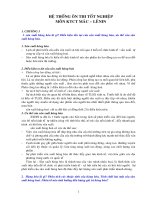
2) Intercept Dummy
An intercept dummy is a variable, says D, has the value of either 0 or 1. It is normally used as a
regressor in the model.

For example, the consumption function (C) can be written as follows:
C = b
0
+ b
1
Y + b
2
D

where
Y is the gross national income
D is equal to 1 for developing countries and 0 for
developed countries
Then,
If D = 0, C = b
0
+ b
1
Y
If D = 1, C = b
0
+ b
1
Y + b
2
D = (b
0
+ b
2
)+ b
1
Y

b
2

C = b
0
+ b

1
Y
C = (b
0
+ b
2
)+ b
1
Y
Y
C


Illustrative example 1 (Maddala, 308)
We suppose that we regress the consumption (C) on income (Y) for household. We include the
following quality variables in the form of dummy variables
Written by Nguyen Hoang Bao May 22, 2004
Applied Econometrics Dummy Variables
2

⎩
⎨
⎧
=
femaleisgenderif0
maleisgenderif1
D
1

⎩
⎨
⎧
<
=
otherwise0
25ageif1
D
2


⎩
⎨
⎧
≤≤
=
otherwise0
50age25if1
D
3


⎩
⎨
⎧
<
=
otherwise0
degreeschoolhigheducationif1
D

4


⎩
⎨
⎧
<≤
=
otherwise0
degreecollegeeducationdegreeschoolhighif1
D
5


Then we run the following regression equation
C = α + βY + γ
1
D
1
+ γ
2
D
2
+ γ
3
D
3
+ γ
4
D

4
+ γ
5
D
5

The assumption made in the dummy variable method is that it is only the intercept that changes for
each group but not the slope coefficient of Y.

Illustrative example 2 (Maddala, 309)
The dummy variable method is also used if one has to take care of seasonal factors. For example, if
we have quarterly data on C and Y, we fit the regression equation

C = α + βY + λ
1
D
1
+ λ
2
D
2
+ λ
3
D
3


where D
1
, D

2
, and D
3
are seasonal dummies defined by:

⎩
⎨
⎧
=
othersfor0
quarterfirstthefor1
D
1


⎩
⎨
⎧
=
othersfor0
quartersecondthefor1
D
2


Written by Nguyen Hoang Bao May 22, 2004
Applied Econometrics Dummy Variables
3
⎩
⎨

⎧
=
othersfor0
quarterthirdthefor1
D
3


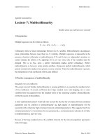
3) Slope Dummy
The slope dummy is defined as an interactive variable.

DY = D x Y
D is equal to 1 for developing countries and 0
for developed countries

Then,
If D = 0, C = b
0
+ b
1
Y
If D = 1, C = b
0
+ b
1
Y + b
2
D = b
0
+(b

1
+ b
2
)Y

C = b
0
+ (b
1
+ b
2
)Y
C = b
0
+ b
1
Y
Y
C



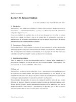
4) Combination of Slope and Intercept Dummies
We may include both slope and intercept dummies in a regression model
DY = D x Y
D is equal to 1 for developing countries and 0 for
developed countries
The general model can be written as follows:
Y = b
0

+ b
1
Y + b
2
D + b
3
DY

Then,
If D = 0, C = b
0
+ b
1
Y
If D = 1, C = b
0
+ b
1
Y + b
2
D = (b
0
+b
2
)+(b
1
+ b
3
)Y
b

2

C = (b
0
+ b
2
) +(b
1
+ b
3
)Y
C = b
0
+ b
1
Y
Y
C

5) Piece – Linear Regression Model
Most of the econometric models we have studied have been continuous, with small changes in one
variable having a measurable effect on another variable.

If we want to explain investment (I) as a function of interest rate (r), the two segments of the
piecewise linear regression show in the below figure.


Written by Nguyen Hoang Bao May 22, 2004
Applied Econometrics Dummy Variables
4

The general model can be written as follows:
I = b
0
+ b
1
r + b
2
(r – r
*
)D
If r < r
*
, then D = 0: I = b
0
+ b
1
r
If r ≥ r
*
, then D = 1: I = b
0
– b
2
r
*
+ (b
1
+ b

2
)r

where r
*
is obtained when we plot the dependent
variable against the explanatory variables and
observing if there seem to be a sharp change in
the relation after a given value of r
*
.
I
r
r
*


6) Summary
If a qualitative variable has m categories, we include (m – 1) dummy variables in the model. The
coefficients attached to the dummy variables must always be interpreted in the relation to the base
variable, that is, the group that gets the value zero.

The use of dummy variables associated with two or more categorical variables allows us to study
partial association and interaction effects in the context of multiple regression. Interactive dummies
are obtained by multiplying dummies corresponding to the different categorical variables. This
allows us to test formally whether interaction is present or not.


References

Bao, Nguyen Hoang (1995), ‘Applied Econometrics’, Lecture notes and Readings,
Vietnam-Netherlands Project for MA Program in Economics of Development.

Maddala, G.S. (1992), ‘Introduction to Econometrics’, Macmillan Publishing Company, New York.

Mukherjee Chandan, Howard White and Marc Wuyts (1998), ‘Econometrics and Data Analysis for
Developing Countries’ published by Routledge, London, UK.

Wonnacott, Thomas H. and Ronald J. Wonnacott (1990). ‘Introductory Statistics’, Published by John
Wiley and Sons, Inc., Printed in the United States of America.

Written by Nguyen Hoang Bao May 22, 2004
Applied Econometrics Dummy Variables
5
Workshop 4: Use of Dummy Variables

1) To help firms determine which of their executive salaries might be out of line, a management
consultant fitted the following multiple regression equation from data base of 270 executives
under the age of 40:

SAL = 43.3 + 1.23 EXP + 3.60 EDUC + 0.74 MALE
(SE) (0.30) (1.20) (1.10)
residual standard deviation s = 16.4
where
SAL = the executive’s annual salary ($000)
EDUC = number of years of post – secondary education
EXP = number of years of experience
MALE = dummy variable, coded 1 for male, 0 for female

1.1) From this regression, a firm can calculate the fitted salary of each of its executives. If the

actual salary is much lower or higher, it can be reviewed to see whether it is appropriate.
Fred Kopp, for example, is a 32 – year old vice president of a large restaurant chain. He
has been with the firm since he obtained a 2 – year MBA at age 25, following a 4 – year
degree in economics. He now earns $126,000 annually.
1.1.1) What is Fred’s fitted salary?
1.1.2) How many standard deviations is his actual salary away from his fitted salary?
Would you therefore call his salary exceptional?
1.1.3) Closer inspection of Fred’s record showed that he had spent two years studying
at Oxford as a Rhodes Scholar before obtaining his MBA. In light of this
information, recalculate your answers to 5.1.1) and 5.1.2)

1.2) In addition to identifying unusual salaries in specific firms, the regression can be used to
answer questions about the economy – wide structure of executive salaries in all firms.
For example,
1.2.1) Is there evidence of sex discrimination?
1.2.2) Is it fair to say that each year’s education (beyond high school) increases the
income of the average executive by $3,600 a year?


Written by Nguyen Hoang Bao May 22, 2004
Applied Econometrics Dummy Variables
6
2) In an environment study of 1072 men, a multiple regression was calculated to show how lung
function was related to several factors, including some hazardous occupations (Lefcoe and
Wonnacott, 1974):

AIRCAP = 4500 – 39 AGE – 9.0 SMOK – 350 CHEMW – 380 FARMW – 180 FIREW
(SE) (1.8) (2.2) (46) (53) (54)

where

AIRCAP = air capacity (milliliters) that the worker can expire in one second
AGE = age (years)
SMOK = amount of current smoking (cigarettes per day)
CHEMW = 1 if subject is a chemical worker, 0 if not
FARMW = 1 if subject is a farm worker, 0 if not
FIREW = 1 if subject is a firefighter, 0 if not

A fourth occupation, physician, served as the reference group, and so did not need a dummy.
Assuming these 1072 people were a random sample,

2.1) Calculate the 95% confidence interval for each coefficient

Fill in the blanks, and choose the correct word in square brackets:

2.2) Other things being equal (things such as _____________), chemical workers on average have
AIRCAP values that are _____________ milliliters [higher, lower] than physicians

2.3) Other things being equal, chemical workers on average have AIRCAP values that are _________
milliliters [higher, lower] than farm workers

2.4) Other things being equal, on average a man who is 1 year older has an AIRCAP value that is
___________ milliliters [higher, lower]

2.5) Other things being equal, on average a man who smokes one pack (20 cigarettes) a day has an
AIRCAP value that is ____________ milliliters [higher, lower]

2.6) As far as AIRCAP is concerned, we estimate that smoking one package a day is roughly
equivalent to aging ___________ years. But this estimate may be biased because of ________
Written by Nguyen Hoang Bao May 22, 2004
Applied Econometrics Dummy Variables

7

3) In an observation study to determine the effect of a drug on blood pressure it was noticed that
the treated group (taking the drug) tended to weigh more than the control group. Thus, when
treated group had higher blood pressure on average, was it because of the treatment or their
weight? To untangle this knot, some regressions were computed, using the following variables:

BP = blood pressure
WEIGHT = weight
D = 1 if taking the drug, 0 otherwise
The data set is given by:
D WEIGHT BP
0
0
0
0
0
0
0
0
0
1
1
1
1
1
1
180
150
210

140
160
160
150
200
160
190
240
200
180
190
220
81
75
83
74
72
80
78
80
74
85
102
95
86
100
90


3.1) How much higher on average would the blood pressure be:

a) For someone of the same weight who is on the drug?
b) For someone on the same treatment who is 10 lbs. heavier?

3.2) How would the simple regression coefficient compare to the multiple regression
coefficient for weight? Why?



Written by Nguyen Hoang Bao May 22, 2004
Applied Econometrics Dummy Variables
8
4) Use data file SRINA

4.1) Regress Ip on Ig

4.2) Repeat the regression using (i) an intercept dummy; (ii) a slope dummy; and, (iii) both
slope and intercept dummies. Select the break point by looking at the scatter plot Ip against
Ig

4.3) Draw scatter plot and fitted line on each regression

4.4) Comment on your results

5) Use data file LEACCESS

5.1) Regress LE on Y

5.2) Repeat the regression using (i) an intercept dummy; (ii) a slope dummy; and, (iii) both
slope and intercept dummies. Use t test check whether they are significant or not. Select
the break point by looking at the scatter plot LE against Y.

5.3) Draw scatter plot and fitted line on each regression

5.4) Comment on your results

6) Use data file AIDSAV

6.1) Regress S/Y on A/Y

6.2) Repeat the regression using dummy variable to take on the distinct value

6.3) Draw the scatter plot and fitted line on each regression

6.4) Comment on your results



Written by Nguyen Hoang Bao May 22, 2004
Applied Econometrics Dummy Variables
9
7) Use data file TOT

7.1) Regress ln(TOT) on t

7.2) Repeat the regression using appropriate dummy

7.3) Draw the time graph of the TOT (not logged) and showing your two fitted line

7.4) Comment on your results

8) Use data file INDIA

8.1) Does your conclusion confirm that gender matter in terms of explaining earning
differences?

8.2) Does your conclusion confirm that educational level in terms of explaining earning
differences?

8.3) Regress ln(WI) on gender, education, and age using the appropriate dummy variables?








Written by Nguyen Hoang Bao May 22, 2004