Tài liệu Process Dynamics, Operations, and Control pptx
Bạn đang xem bản rút gọn của tài liệu. Xem và tải ngay bản đầy đủ của tài liệu tại đây (2.96 MB, 179 trang )
Spring 2006 Process Dynamics, Operations, and Control 10.450
Lesson 1: Processes and Systems
1.0 context and direction
Process control is an application area of chemical engineering - an
identifiable specialty for the ChE. It combines chemical process
knowledge (how physics, chemistry, and biology work in operating
equipment) and an understanding of dynamic systems, a topic important to
many fields of engineering. Thus study of process control allows
chemical engineers to span their own field, as well as form a useful
acquaintance with allied fields. Practitioners of process control find their
skills useful in design, operation, and troubleshooting - major categories of
chemical engineering practice.
Process control, like any coherent topic, is an integrated body of
knowledge - it hangs together on a multidimensional framework, and
practitioners draw from many parts of the framework in doing their work.
Yet in learning, we must receive information in sequence - following a
path through multidimensional space. It is like entering a large building
with unlighted rooms, holding a dim flashlight and clutching a vague map
that omits some of the stairways and passages. How best to learn one’s
way around?
In these lessons we will attempt to move through a significant portion of
the structure - say, half a textbook - in about two weeks. Then we will
repeat the journey several times, each time inspecting the rooms more
thoroughly. By this means we hope to gain, from the start, a sense of
doing an entire process control job, as well as approach each new topic in
the context of a familiar path.
1.1 the job we will do, over and over
We encounter a process, learn how it behaves, specify how we wish to
control it, choose appropriate equipment, and then explore the behavior
under control to see if we have improved things.
1.2 introducing a simple process
A large tank must be filled with liquid from a supply line. One operator
stands at ground level to operate the feed valve. Another stands on the
tank, gauging its level with a dipstick. When the tank is near full, the stick
operator will instruct the other to start closing the valve. Overfilling can
cause spills, but underfilling will cause later process problems.
revised 2006 Jan 30 1
Spring 2006 Process Dynamics, Operations, and Control 10.450
Lesson 1: Processes and Systems
To learn how the process works, we write an overall material balance on
the tank.
i
FV
dt
d
ρ=ρ
(1.2-1)
The tank volume V can be expressed in terms of the liquid level h. The
inlet volumetric flow rate F
i
may vary with time due to supply pressure
fluctuations and valve manipulations by the operator. The liquid density
depends on the temperature, but will usually not vary significantly with
time during the course of filling. Thus (1.2-1) becomes
)t(F
d
t
dh
A
i
=
(1.2-2)
We integrate (1.2-2) to find the liquid level as a function of time.
∫
+=
t
0
i
dt)t(F
A
1
)0(hh
(1.2-3)
1.3 planning a control scheme
Clearly the liquid level h is important, and we will call it the controlled
variable. Our control objective is to bring h quickly to its target value h
r
and not exceed it. (To be realistic, we would specify allowable limits ± δh
on h
r
.) We will call the volumetric flow F
i
the manipulated variable,
because we adjust it to achieve our objective for the controlled variable.
The existing control scheme is to measure the controlled variable via
dipstick, decide when the controlled variable is near target, and instruct
revised 2006 Jan 30 2
Spring 2006 Process Dynamics, Operations, and Control 10.450
Lesson 1: Processes and Systems
the valve operator to change the manipulated variable. The scheme suffers
from
• delay in measurement. Overfilling can occur if the stick operator
cannot complete the measurement in time.
• performance variations. Both stick and valve operators may vary in
attentiveness and speed of execution.
• resources required. There are better uses for operating personnel.
• unsafe conditions. There is too much potential for chemical exposure.
A new scheme is proposed: put a timer on the valve. Calculate the time
required for filling from (1.2-3). Close the valve when time has expired.
The timing scheme would no longer require an operator to be on the tank
top, and with a motor-driven valve actuator the entire operation could be
directed from a control room. These are indeed improvements. However,
the timing scheme abandons a crucial virtue of the existing scheme: by
measuring the controlled variable, the operators can react to unexpected
disturbances, such as changes in the filling rate. Using knowledge of the
controlled variable to motivate changes to the manipulated variable is a
fundamental control structure, known as feedback control
. The proposed
timing scheme has no feedback mechanism, and thus cannot accommodate
changes to h(0) and F
i
(t) in (1.2-3).
An alternative is to build on the feedback already inherent in the two-
operator scheme, but to improve its operation. We propose an automatic
controller that behaves according to the following controller algorithm:
near i max
r
near i max
r near
hh F F
hh
hh FF
hh
<=
−
>=
−
(1.3-1)
Algorithm (1.3-1) is an idealization of what the operators are already
doing: filling occurs at maximum flow until the level reaches a value h
near
.
Beyond this point, the flow decreases linearly, reaching zero when h
reaches the target h
r
. The setting of h
near
may be adjusted to tune the
control performance.
1.4 choosing equipment
We need a sensor to replace the dipstick, a valve actuator to replace the
valve operator, and a controller mechanism to replace the stick operator.
We imagine a buoyant object floating on the liquid surface. The float is
linked to a lever that drives the valve stem. When the liquid level is low,
the float rests above it on a structure so that the valve is fully open.
revised 2006 Jan 30 3
Spring 2006 Process Dynamics, Operations, and Control 10.450
Lesson 1: Processes and Systems
1.5 process behavior under automatic control
Typically these things work quite well. We predict its performance by
combining our process model (1.2-2) with the controller algorithm (1.3-1),
which eliminates the manipulated variable between the equations. We
take the simple case in which F
max
does not vary during filling due to
pressure fluctuations, etc. For h less than h
near
,
t
A
F
)0(hh
known)0(hF
dt
dh
A
max
max
+=
==
(1.5-1)
Equation (1.5-1) can be used to calculate t
near
, the time at which h reaches
h
near
. For h greater than h
near
,
()
()
r
max near near
rnear
r near
r r near
fill r near
hhdh
AF h(t)h
dt h h
h(t t )
hh h h exp
thh
−
==
−
⎡
−−
=− −
⎢⎥
−
⎢⎥
⎣⎦
⎤
(1.5-2)
revised 2006 Jan 30 4
Content removed due to copyright restrictions.
(To see a cut-away diagram of a toilet, go to
/>Spring 2006 Process Dynamics, Operations, and Control 10.450
Lesson 1: Processes and Systems
where the parameter t
fill
is the time required for the level to reach h
r
at
flow F
max
, starting from an empty tank.
r
fill
max
Ah
t
F
=
(1.5-3)
The plot shows the filling profile from h(0) = 0.10h
r
with several values of
h
near
/h
r
. Certainly the filling goes faster if the flow can go instantaneously
from F
max
to zero at h
r
; however this will not be practical, so that h
near
will
be less than h
r
.
0
0.2
0.4
0.6
0.8
1
1.2
0 0.2 0.4 0.6 0.8 1 1.2 1.4
t/t
fill
h/hr
h
near
/h
r
= 0.95
0.75
0.50
0
0.2
0.4
0.6
0.8
1
1.2
0 0.2 0.4 0.6 0.8 1 1.2 1.4
t/t
fill
h/hr
h
near
/h
r
= 0.95
0.75
0.50
1.6 defining ‘system’
In Section 1.2, we introduced a process - a tank with feed piping - whose
inventory varied in time. We thought of the process as a collection of
equipment and other material, marked off by a boundary in space,
communicating with its environment by energy and material streams.
'Process' is a good notion, important to chemical engineers. Another
useful notion is that of 'system'. A system is some collection of equipment
and operations, usually with a boundary, communicating with its
environment by a set of input and output signals. By these definitions, a
process is a type of system, but system is more abstract and general. For
example, the system boundary is often tenuous: suppose that our system
comprises the equipment in the plant and the controller in the central
control room, with radio communication between the two. A physical
boundary would be in two pieces, at least; perhaps we should regard this
revised 2006 Jan 30 5
Spring 2006 Process Dynamics, Operations, and Control 10.450
Lesson 1: Processes and Systems
system boundary as partly physical (around the chemical process) and
partly conceptual (around the controller).
Furthermore, the inputs and outputs of a system need not be material and
energy streams, as they are for a process. System inputs are "things that
cause" or “stimuli”; outputs are "things that are affected" or “responses”.
system
inputs
(causes)
outputs
(responses)
To approach the problem of controlling our filling process in Section 1.3,
we thought of it in system terms: the primary output was the liquid level h
not a stream, certainly, but an important response variable of the system
and inlet stream F
i
was an input. And peculiar as it first seems, if the
tank had an outlet flow F
o
, it would also be an input signal, because it
influences the liquid level, just as does F
i
.
The point of all this is to look at a single schematic and know how to view
it as a process, and as a system. View it as a process (F
o
as an outlet
stream) to write the material balance and make fluid mechanics
calculations. View it as a system (F
o
as an input) to analyze the dynamic
behavior implied by that material balance and make control calculations.
System dynamics is an engineering science useful to mechanical,
electrical, and chemical engineers, as well as others. This is because
transient behavior, for all the variety of systems in nature and technology,
can be described by a very few elements. To do our job well, we must
understand more about system dynamics how systems behave in time.
That is, we must be able to describe how important output variables react
to arbitrary disturbances.
1.7 systems within systems
We call something a system and identify its inputs and outputs as a first
step toward understanding, predicting, and influencing its behavior. In
some cases it may help to determine some of the structure within the
system boundaries; that is, if we identify some
component systems. Each
of these, of course, would have inputs and outputs, too.
system
inputs outputs
1
2
revised 2006 Jan 30 6
Spring 2006 Process Dynamics, Operations, and Control 10.450
Lesson 1: Processes and Systems
Considering the relationship of these component systems, we recognize
the existence of
intermediate variables within a system. Neither inputs
nor outputs of the main system, they connect the component systems.
Intermediate variables may be useful in understanding and influencing
overall system behavior.
1.8 the system of single-loop feedback control
When we add a controller to a process, we create a single time-varying
system; however, it is useful to keep process and controller conceptually
distinct as component systems. This is because a repertoire of relatively
few control schemes (relationships between process and controller)
suffices for myriad process applications. Using the terms we defined in
Section 1.3, we represent a control scheme called
single-loop feedback
control
in this fashion:
process
controller
final control
element
sensor
set point
manipulated
variable
other inputs other
outputs
controlled
variable
system
process
controller
final control
element
sensor
set point
manipulated
variable
other inputs other
outputs
controlled
variable
system
Figure 1.8-1 The single-loop feedback control system and its
subsystems
We will see this structure repeatedly. Inside the block called "process" is
the physical process, whatever it might be, and the block is the boundary
we would draw if we were doing an overall material or energy balance.
HOWEVER, we remember that the inputs and outputs are NOT
necessarily the same as the material and energy streams that cross the
process boundary. From among the outputs, we may select a controlled
variable (often a pressure, temperature, flow rate, liquid level, or
composition) and provide a suitable sensor to measure it. From the inputs,
we choose a manipulated variable (often a flow rate) and install an
appropriate final control element (often a valve). The measurement is fed
to the controller, which decides how to adjust the manipulated variable to
keep the controlled variable at the desired condition: the set point. The
revised 2006 Jan 30 7
Spring 2006 Process Dynamics, Operations, and Control 10.450
Lesson 1: Processes and Systems
other inputs are potential disturbances that affect the controlled variable,
and so require action by the controller.
1.9 conclusion
Think of a chemical process as a dynamic system that responds in
particular ways to its inputs. We attach other dynamic systems (sensor,
controller, etc.) to that process in a single-loop feedback structure and
arrive at a new dynamic system that responds in different ways to the
inputs. If we do our job well, it responds in better
ways, so to justify all
the trouble.
revised 2006 Jan 30 8
Spring 2006 Process Dynamics, Operations, and Control 10.450
Lesson 2: Mathematics Review
2.0 context and direction
Imagine a system that varies in time; we might plot its output vs. time. A
plot might imply an equation, and the equation is usually an ODE
(ordinary differential equation). Therefore, we will review the math of the
first-order ODE while emphasizing how it can represent a dynamic
system. We examine how the system is affected by its initial condition
and by disturbances, where the disturbances may be non-smooth, multiple,
or delayed.
2.1 first-order, linear, variable-coefficient ODE
The dependent variable y(t) depends on its first derivative and forcing
function x(t). When the independent variable t is t
0
, y is y
0
.
00
y)t(y)t(Kx)t(y
d
t
dy
)t(a ==+
(2.1-1)
In writing (2.1-1) we have arranged a coefficient of +1 for y. Therefore
a(t) must have dimensions of independent variable t, and K has
dimensions of y/x. We solve (2.1-1) by defining the integrating factor p(t)
∫
=
)(
exp)(
ta
dt
tp (2.1-2)
Notice that p(t) is dimensionless, as is the quotient under the integral. The
solution
∫
+=
t
t
00
0
dt
)t(a
)t(x)t(p
)t(p
K
)t(p
)t(y)t(p
)t(y (2.1-3)
comprises contributions from the initial condition y(t
0
) and the forcing
function Kx(t). These are known as the homogeneous (as if the right-hand
side were zero) and particular (depends on the right-hand side) solutions.
In the language of dynamic systems, we can think of y(t) as the response
of the system to input disturbances Kx(t) and y(t
0
).
2.2 first-order ODE, special case for process control applications
The independent variable t will represent time. For many process control
applications, a(t) in (2.1-1) will be a positive constant; we call it the time
constant τ.
00
y)t(y)t(Kx)t(y
dt
dy
==+τ
(2.2-1)
The integrating factor (2.1-2) is
revised 2005 Jan 11 1
Spring 2006 Process Dynamics, Operations, and Control 10.450
Lesson 2: Mathematics Review
τ
=
τ
=
∫
t
e
dt
exp)t(p
(2.2-2)
and the solution (2.1-3) becomes
()
dt)t(xee
K
ey)t(y
t
t
tt
tt
0
0
0
∫
ττ
−
τ
−−
τ
+= (2.2-3)
The initial condition affects the system response from the beginning, but
its effect decays to zero according to the magnitude of the time constant -
larger time constants represent slower decay. If not further disturbed by
some x(t), the first order system reaches equilibrium at zero.
However, most practical systems are disturbed. K is a property of the
system, called the gain. By its magnitude and sign, the gain influences
how strongly y responds to x. The form of the response depends on the
nature of the disturbance.
Example: suppose x is a unit step function at time t
1
. Before we proceed
formally, let us think intuitively. From (2.2-3) we expect the response y to
decay toward zero from IC y
0
. At time t
1
, the system will respond to being
hit with a step disturbance. After a long time, there will be no memory of
the initial condition, and the system will respond only to the disturbance
input. Because this is constant after the step, we guess that the response
will also become constant.
Now the math: from (2.2-3)
()
()
()
⎟
⎠
⎞
⎜
⎝
⎛
−−+=
−
τ
+=
τ
−−
τ
−−
ττ
−
τ
−−
∫
1
0
0
0
tt
1
tt
0
t
t
1
tt
tt
0
e1)tt(KUey
dt)tt(Uee
K
ey)t(y
(2.2-4)
Figure 2.2-1 shows the solution. Notice that the particular solution makes
no contribution before time t
1
. The initial condition decays, and with no
disturbance would continue to zero. At t
1
, however, the system responds
to the step disturbance, approaching constant value K as time becomes
large. This immediate response, followed by asymptotic approach to the
new steady state, is characteristic of first-order systems. Because the
response does not track the step input faithfully, the response is said to lag
behind the input; the first-order system is sometimes called a first-order
lag.
revised 2005 Jan 11 2
Spring 2006 Process Dynamics, Operations, and Control 10.450
Lesson 2: Mathematics Review
0
0.5
1
012345
disturbance
6
0
0.5
1
1.5
2
2.5
0123456
time
response
t
0
t
1
y
0
K
0
0.5
1
012345
disturbance
6
0
0.5
1
1.5
2
2.5
0123456
time
response
t
0
t
1
y
0
K
Figure 2.2-1 first-order response to initial condition and step
disturbance
2.3 piecewise integration of non-smooth disturbances
The solution (2.2-3) is applied over succeeding time intervals, each
featuring an initial condition (from the preceding interval) and disturbance
input.
()
()
⎪
⎪
⎪
⎪
⎩
⎪
⎪
⎪
⎪
⎨
⎧
<<
τ
+
<<
τ
+
=
∫
∫
ττ
−
τ
−−
ττ
−
τ
−−
.etc
tttdt)t(xee
K
e)t(y
tttdt)t(xee
K
e)t(y
)t(y
21
t
t
tt
tt
1
10
t
t
tt
tt
0
1
1
0
0
(2.3-1)
Example: suppose
revised 2005 Jan 11 3
Spring 2006 Process Dynamics, Operations, and Control 10.450
Lesson 2: Mathematics Review
()
⎪
⎩
⎪
⎨
⎧
<
<<−
<<
=
==+
t20
2t11t2
1t00
x
0)0(yxy
dt
dy
(2.3-2)
In this problem, variables t, x, and y should be presumed to have
appropriate, if unstated, units; in these units, both gain and time constant
are of magnitude 1. From (2.3-1),
()
()
()
⎪
⎩
⎪
⎨
⎧
<
<<+−
<<
=
−−−
−−
t2ee2
2t1e2t2
1t00
)t(y
2t1
1t
(2.3-3)
With a zero initial condition and no disturbance, the system remains at
equilibrium until the ramp disturbance begins at t = 1. Then the output
immediately rises in response, lagging behind the linear ramp. At t = 2,
the disturbance ceases, and the output decays back toward equilibrium.
revised 2005 Jan 11 4
Spring 2006 Process Dynamics, Operations, and Control 10.450
Lesson 2: Mathematics Review
0
0.5
1
1.5
2
2.5
012345
disturbance
6
0
0.1
0.2
0.3
0.4
0.5
0.6
0.7
0.8
0123456
time
response
0
0.5
1
1.5
2
2.5
012345
disturbance
6
0
0.1
0.2
0.3
0.4
0.5
0.6
0.7
0.8
0123456
time
response
2.4 multiple disturbances and superimposition
Systems can have more than one input. Consider a first-order system with
two disturbance functions.
002211
y)t(y)t(xK)t(xK)t(y
dt
dy
=+=+τ
(2.4-1)
Applying (2.2-3) and distributing the integral across the disturbances, we
find that the effects of the disturbances on y are additive.
()
dt)t(xee
K
dt)t(xee
K
ey)t(y
2
t
t
tt
2
1
t
t
tt
1
tt
0
00
0
∫∫
ττ
−
ττ
−
τ
−−
τ
+
τ
+=
(2.4-2)
This additive behavior is a happy characteristic of linear systems. Thus
another way to view problem (2.4-1) is to decompose it into component
problems. That is, define
21H
yyyy ++=
(2.4-3)
revised 2005 Jan 11 5
Spring 2006 Process Dynamics, Operations, and Control 10.450
Lesson 2: Mathematics Review
and write (2.4-1) in three equations. We put the initial condition with no
disturbances, and each disturbance with a zero initial condition.
0)t(y)t(xK)t(y
d
t
dy
0)t(y)t(xK)t(y
dt
dy
y)t(y0)t(y
dt
dy
02222
2
01111
1
00HH
H
==+τ
==+τ
==+τ
(2.4-4)
Equations and initial conditions (2.4-4) can be summed to recover the
original problem specification (2.4-1). The solutions are
()
dt)t(xee
K
)t(y
dt)t(xee
K
)t(y
ey)t(y
2
t
t
tt
2
2
1
t
t
tt
1
1
tt
0H
0
0
0
∫
∫
ττ
−
ττ
−
τ
−−
τ
=
τ
=
=
(2.4-5)
and of course these solutions can be added to recover original solution
(2.4-2). Thus we can view the problem of multiple disturbances as a
system responding to the sum of the disturbances, or as the sum of
responses from several identical systems, each responding to a single
disturbance.
Example: consider
2)0(y)3t(U)1t(U
4
3
y
4
1
dt
dy
4
1
=−−−=+
(2.4-6)
We first place the equation in standard form, in which the coefficient of y
is +1.
2)0(y)3t(U4)1t(U3y
d
t
dy
=−−−=+
(2.4-7)
Equation (2.4-7) shows us that the time constant is 1, and that the system
responds to the first disturbance with a gain of 3, and to the second with a
gain of -4. The solution is
(
)
(
)
)3t()1t(t
e1)3t(U4e1)1t(U3e2y
−−−−−
−−−−−+= (2.4-8)
revised 2005 Jan 11 6
Spring 2006 Process Dynamics, Operations, and Control 10.450
Lesson 2: Mathematics Review
In Figure 2.4-1, the individual solution components are plotted as solid
traces; their sum, which is the system response, is a dashed trace. Notice
how the first-order lag responds to each new disturbance as it occurs.
0
0.5
1
0246
disturbances
8
-5
-4
-3
-2
-1
0
1
2
3
4
0246
time
response
8
0
0.5
1
0246
disturbances
8
-5
-4
-3
-2
-1
0
1
2
3
4
0246
time
response
8
)
Figure 2.4-1 first-order response to multiple disturbances
Writing the step functions explicitly in solution (2.4-8) emphasizes that
particular disturbances do not influence the solution until the time of their
occurrence. For example, if they were omitted, some
deceptively correct
but inappropriate
rearrangement would lead to errors.
()(
)3t()1t(t
)3t()1t(t
)3t()1t(t
e4e3e21
e44e33e2
e14e13e2y
−−−−−
−−−−−
−−−−−
+−+−=
+−−+=
−−−+=
(do not do this!) (2.4-9)
This notation at least implies that two of the exponential functions have
delayed onsets. However, further correct-but-inappropriate rearrangement
makes things even worse.
revised 2005 Jan 11 7
Spring 2006 Process Dynamics, Operations, and Control 10.450
Lesson 2: Mathematics Review
()
t31
t3t1t
)3t()1t(t
ee4e321
ee4ee3e21
e4e3e21y
−
−−−
−−−−−
+−+−=
+−+−=
+−+−=
(do not do this!) (2.4-10)
The incorrect solutions are plotted with (2.4-8) in Figure 2.4-2. Equation
(2.4-9) has become discontinuous - the response takes non-physical leaps
at the onset of each new disturbance. Equation (2.4-10) has lost all
dependence on the disturbances and decays from a non-physical initial
condition. Even with the mistakes, both incorrect solutions lead to the
correct long-term condition.
-5
0
5
10
15
20
0246
time
response
8
solution eq 2.4.9 eq 2.4.10
Figure 2.4-2 comparison of correct and incorrect solutions
2.5 delayed response to disturbances
Consider a system that reacts to a disturbance, but only after some
intervening time interval θ has passed. That is
00
y)t(y)t(Kx)t(y
dt
dy
=θ−=+τ
(2.5-1)
Equation (2.5-1) shows the dependence of y, at any time t, on the value of
x at earlier time t - θ. The solution is written directly from (2.2-3).
()
dt)t(xee
K
ey)t(y
t
t
tt
tt
0
0
0
θ−
τ
+=
∫
ττ
−
τ
−−
(2.5-2)
We must integrate the disturbance considering the time delay. Take as an
example a disturbance x(t) occurring at time t
1
. The plot shows the
revised 2005 Jan 11 8
Spring 2006 Process Dynamics, Operations, and Control 10.450
Lesson 2: Mathematics Review
disturbance, as well as the disturbance as the system experiences it, which
begins at time t
1
+ θ. We could express this disturbance-as-experienced as
some new function x
1
(t), occurring at time t
1
+ θ.
t
0
t
1
t
1
+ θ
t
0
- θ
t
1
ξ
t
t
1
- θ
disturbance
as it occurs
disturbance as
experienced by
system
x(t) x(t - θ) = x
1
(t)
x(ξ)
t
0
t
1
t
1
+ θ
t
0
- θ
t
1
ξ
t
t
1
- θ
disturbance
as it occurs
disturbance as
experienced by
system
x(t) x(t - θ) = x
1
(t)
x(ξ)
Alternatively, we could define a new time variable
θ−=ξ t
(2.5-3)
and write the input as x(ξ). The integral in (2.5-2) becomes, then,
ξξ==θ−
∫∫∫
ξ
θ−
τ
θ+ξ
ττ
d)(xedt)t(xedt)t(xe
000
t
1
t
t
t
t
t
t
(2.5-4)
Therefore, solution (2.5-2) becomes
()
ξξ
τ
+=
∫
ξ
θ−
τ
ξ
τ
θ
τ
−
τ
−−
d)(xeee
K
ey)t(y
0
0
t
t
tt
0
(2.5-5)
Example: consider a step disturbance at time t = 2 that affects the system
3 time units later.
)2t(U)t(x
0)0(y)3t(xy
dt
dy
−=
=−=+
(2.5-6)
Using (2.5-5)
revised 2005 Jan 11 9
Spring 2006 Process Dynamics, Operations, and Control 10.450
Lesson 2: Mathematics Review
[]
[]
[]
)5t(
3t23t3t
23t3t
2
3t
2
2
30
3t
30
3t
e1)5t(U
ee)5t(U
eeee)23t(U
e)2(Uee
d)2(Ued)2(Ueee
d)2(Ueeey
−−
+−+−−
−−
ξ
ξ−
ξ
ξ
−
ξ−
ξ
−
ξ−
−−=
−−=
−−−=
⎥
⎦
⎤
⎢
⎣
⎡
−ξ=
⎥
⎥
⎦
⎤
⎢
⎢
⎣
⎡
ξ−ξ+ξ−ξ=
ξ−ξ=
∫∫
∫
(2.5-7)
Figure 2.5-1 shows that a typical first-order lag step response occurs 3
time units after being disturbed at t = 2.
0
0.5
1
024681
disturbances
0
0
0.2
0.4
0.6
0.8
1
024681
time
response
0
0
0.5
1
024681
disturbances
0
0
0.2
0.4
0.6
0.8
1
024681
time
response
0
Figure 2.5-1 step response of first order system with dead time
The time delay in responding to a disturbance is often called dead time
.
Dead time is different from lag. Lag occurs because of the combination of
y and its derivative on the left-hand side of the equation. Dead time
revised 2005 Jan 11 10
Spring 2006 Process Dynamics, Operations, and Control 10.450
Lesson 2: Mathematics Review
occurs because of a time delay in processing a disturbance on the right-
hand side.
2.6 conclusion
Please become comfortable with handling ODEs. View them as systems;
identify their inputs and outputs, their gains and time parameters.
revised 2005 Jan 11 11
Spring 2006 Process Dynamics, Operations, and Control 10.450
Lesson 3: The Blending Tank
3.0 context and direction
A particularly simple process is a tank used for blending. Just as promised
in Section 1.1, we will first represent the process as a dynamic system and
explore its response to disturbances. Then we will pose a feedback control
scheme. We will briefly consider the equipment required to realize this
control. Finally we will explore its behavior under control.
DYNAMIC SYSTEM BEHAVIOR
3.1 math model of a simple continuous holding tank
Imagine a process stream comprising an important chemical species A in
dilute liquid solution. It might be the effluent of some process, and we
might wish to use it to feed another process. Suppose that the solution
composition varies unacceptably with time. We might moderate these
swings by holding up a volume in a stirred tank: intuitively we expect the
changes in the outlet composition to be more moderate than those of the
feed stream.
F, C
Ai
F, C
Ao
volume V
F, C
Ai
F, C
Ao
volume V
Our concern is the time-varying behavior of the process, so we should
treat our process as a dynamic system. To describe the system, we begin
by writing a component material balance over the solute.
AoAiAo
FCFCVC
dt
d
−=
(3.1-1)
In writing (3.1-1) we have recognized that the tank operates in overflow:
the volume is constant, so that changes in the inlet flow are quickly
duplicated in the outlet flow. Hence both streams are written in terms of a
single volumetric flow F. Furthermore, for now we will regard the flow as
constant in time.
Balance (3.1-1) also represents the concentration of the outlet stream, C
Ao
,
as the same as the average concentration in the tank. That is, the tank is a
perfect mixer: the inlet stream is quickly dispersed throughout the tank
volume. Putting (3.1-1) into standard form,
revised 2005 Jan 13 1
Spring 2006 Process Dynamics, Operations, and Control 10.450
Lesson 3: The Blending Tank
AiAo
Ao
CC
dt
dC
F
V
=+
(3.1-2)
we identify a first-order dynamic system describing the response of the
outlet concentration C
Ao
to disturbances in the inlet concentration C
Ai
.
The speed of response depends on the time constant, which is equal to the
ratio of tank volume and volumetric flow. Although both of these
quantities influence the dynamic behavior of the system, they do so as a
ratio. Hence a small tank and large tank may respond at the same rate, if
their flow rates are suitably scaled.
System (3.1-2) has a gain equal to 1. This means that a sustained
disturbance in the inlet concentration is ultimately communicated fully to
the outlet.
Before solving (3.1-2) we specify a reference condition: we prefer that C
Ao
be at a particular value C
Ao,r
. For steady operation in the desired state,
there is no accumulation of solute in the tank.
r,Aor,Ai
r
Ao
CC0
dt
dC
F
V
−==
(3.1-3)
Thus, as expected, steady outlet conditions require a steady inlet at the
same concentration; call it C
A,r
. Let us take this reference condition as an
initial condition in solving (3.1-2). The solution is
dt)t(Ce
e
eC)t(C
Ai
t
0
t
t
t
r,AAo
∫
τ
τ
−
τ
−
τ
+=
(3.1-4)
where the time constant is
F
V
=τ
(3.1-5)
Equation (3.1-4) describes how outlet concentration C
Ao
varies as C
Ai
changes in time. In the next few sections we explore the transient
behavior predicted by (3.1-4).
3.2 response of system to steady input
Suppose inlet concentration remains steady at C
A,r
. Then from (3.1-4)
revised 2005 Jan 13 2
Spring 2006 Process Dynamics, Operations, and Control 10.450
Lesson 3: The Blending Tank
r,A
tt
r,A
t
r,A
t
0
t
r,A
t
t
r,AAo
C1eeCeC
eC
e
eCC
=
⎟
⎠
⎞
⎜
⎝
⎛
−+=
τ
τ
+=
ττ
−
τ
−
τ
τ
−
τ
−
(3.2-1)
Equation (3.2-1) merely confirms that the system remains steady if not
disturbed.
3.3 leaning on the system - response to step disturbance
Step functions typify disturbances in which an input variable moves
relatively rapidly to some new value and remains there. Suppose that
input C
Ai
is initially at the reference value C
A,r
and changes at time t
1
to
value C
A1
. Until t
1
the outlet concentration is given by (3.2-1). From the
step at t
1
, the outlet concentration begins to respond.
⎟
⎠
⎞
⎜
⎝
⎛
−+=
⎟
⎠
⎞
⎜
⎝
⎛
−+=
>τ
τ
+=
τ
−−
τ
−−
τττ
−
τ
−−
τ
τ
−
τ
−−
)tt(
1A
)tt(
r,A
t
tt
1A
)tt(
r,A
1
t
t
t
1A
t
)tt(
r,AAo
11
11
1
1
e1CeC
eeeCeC
tteC
e
eCC
(3.3-1)
In Figure 3.3-1, C
A,r
= 1 and C
A1
= 0.8 in arbitrary units; t
1
has been set
equal to τ. At sufficiently long time, the initial condition has no influence
and the outlet concentration becomes equal to the new inlet concentration.
After time equal to three time constants has elapsed, the response is about
95% complete – this is typical of first-order systems.
In Section 3.1, we suggested that the tank would mitigate the effect of
changes in the inlet composition. Here we see that the tank will not
eliminate a step disturbance, but it does soften its arrival.
revised 2005 Jan 13 3
Spring 2006 Process Dynamics, Operations, and Control 10.450
Lesson 3: The Blending Tank
0.7
0.8
0.9
1
1.1
012345
t/τ
response
6
0
0.5
1
012345
disturbance
6
Figure 3.3-1 first-order response to step disturbance
3.4 kicking the system - response to pulse disturbance
Pulse functions typify disturbances in which an input variable moves
relatively rapidly to some new value and subsequently returns to normal.
Suppose that C
Ai
changes to C
A1
at time t
1
and returns to C
A,r
at t
2
. Then,
drawing on (3.2-1) and (3.3-1),
⎪
⎪
⎪
⎩
⎪
⎪
⎪
⎨
⎧
<
⎟
⎠
⎞
⎜
⎝
⎛
−+
⎥
⎦
⎤
⎢
⎣
⎡
⎟
⎠
⎞
⎜
⎝
⎛
−+
<<
⎟
⎠
⎞
⎜
⎝
⎛
−+
<<
=
τ
−−
τ
−−
τ
−−
τ
−−
τ
−−
τ
−−
tte1Cee1CeC
ttte1CeC
tt0C
C
2
)tt(
r,A
)tt()tt(
1A
)tt(
r,A
21
)tt(
1A
)tt(
r,A
1r,A
Ao
221212
11
(3.4-1)
In Figure 3.4-1, C
A,r
= 0.6 and C
A1
= 1 in arbitrary units; t
1
has been set
equal to τ and t
2
to 2.5τ. We see that the tank has softened the pulse and
reduced its peak value. A pulse is a sequence of two counteracting step
changes. If the pulse duration is long (compared to the time constant τ),
revised 2005 Jan 13 4
Spring 2006 Process Dynamics, Operations, and Control 10.450
Lesson 3: The Blending Tank
the system can complete the first step response before being disturbed by
the second.
0.4
0.6
0.8
1
012345
t/τ
response
6
0
0.5
1
012345
disturbance
6
Figure 3.4-1 first-order response to pulse disturbance
3.5 shaking the system - response to sine disturbance
Sine functions typify disturbances that oscillate. Suppose the inlet
concentration varies around the reference value with amplitude A and
frequency ω, which has dimensions of radians per time.
()
tsinACC
r,AAi
ω+=
(3.5-1)
From (3.1-4),
()
(
)
ωτ−+ω
τω+
+
τω+
ωτ
−=
−
τ
−
1
22
t
22
r,AAo
tantsin
1
A
e
1
A
CC
(3.5-2)
revised 2005 Jan 13 5
Spring 2006 Process Dynamics, Operations, and Control 10.450
Lesson 3: The Blending Tank
Solution (3.5-2) comprises the mean value C
A,r
, a term that decays with
time, and a continuing oscillation term. Thus, the long-term system
response to the sine input is to oscillate at the same frequency ω. Notice,
however, that the amplitude of the output oscillation is diminished by the
square-root term in the denominator. Notice further that the outlet
oscillation lags the input by a phase angle tan
-1
(-ωτ).
In Figure 3.5-1, C
A,r
= 0.8 and A = 0.5 in arbitrary units; ωτ has been set
equal to 2.5 radians, and τ to 1 in arbitrary units. The decaying portion of
the solution makes a negligible contribution after the first cycle. The
phase lag and reduced amplitude of the solution are evident; our tank has
mitigated the inlet disturbance.
0
0.2
0.4
0.6
0.8
1
1.2
1.4
0246
t/τ
input and response
8
input decaying part continuing part solution
Figure 3.5-1 first-order response to sine disturbance
3.6 frequency response and the Bode plot
The long-term response to a sine input is the most important part of the
solution; we call it the frequency response
of the system. We will
examine the frequency response for an abstract first order system.
(Because we wish to focus on the oscillatory response, we will write (3.6-
1) so that x and y vary about zero. The effect of a non-zero bias term can
be seen in (3.5-1) and (3.5-2).)
revised 2005 Jan 13 6