Tài liệu SPACE, TIME, FRAME, CINEMA EXPLORING THE POSSIBILITIES OF SPATIOTEMPORAL EFFECTS pdf
Bạn đang xem bản rút gọn của tài liệu. Xem và tải ngay bản đầy đủ của tài liệu tại đây (541.48 KB, 13 trang )
1
Space, Time, Frame, Cinema
Exploring the Possibilities of Spatiotemporal Effects
Mark J. P. Wolf
Along with the growth of digital special effects technology, there seems to be a renewed interest in physical
camerawork and the way in which physical cameras can be extended by and combined with virtual cameras.
Without a systematized method of study, however, many possibilities may remain overlooked. This essay
attempts to suggest such a method, and its scope will be limited to the spatial and temporal movements of the
camera.
Without a deliberate method, the discovery of new effects is somewhat haphazard and may take much longer
than it would otherwise. Consider, for example, Edweard Muybridge’s experiments in sequential photography.
In 1877, for his famous attempt to record the movements of a galloping horse, he lined up a row of still cameras
attached to tripwires designed to activate them. But supposing Muybridge had set the camera in a semicircle,
with all the tripwires connected and activated at the same time? [see Fig. 1]
In doing so, the tripwires would have activated all the cameras simultaneously, and since they would all be
aimed at the same point, all the photographs would have shown the horse at the same instant, albeit from a
series of different angles. Had these images been projected in sequence, Muybridge would have discovered the
frozen time effect (or temps mort, as it is known in France) more than a century earlier than it was. Muybridge
actually did set his cameras in a semicircle for certain motion studies, but he did not animate them or exploit the
possibilities of frozen time shots.
1
Fig. 1. A Muybridge set-up (in which a linear camera array
follows a moving subject) versus a Frozen time set-up (in which
a circular camera array tracks around frozen action).
2
Since frozen time effects were possible even in Muybridge’s day, why did it take over a century for them to
be discovered? What other potential effects are still out there in the realm of possibility, waiting to be
discovered and exploited? A systemized study of spatiotemporal effects is one way to look for gaps that may
aid in the discovery of new effects.
The potential existence of the frozen time effect could have been found through a consideration of the
possible ways one can combine camera movements in space and time [see Fig. 2].
The first variable is that of movement, which is either present or not present.
Applied to space, this gives us
moving camera shots and static camera shots. Applied to time, this gives us motion pictures and still
photographs, or for short, shots and stills, where a shot consists of a series of stills. Combining both spatial and
temporal variables gives us four motion picture possibilities.
A moving camera shot occurs when a camera is both moving through space and moving through time; that
is, recording a series of images which are temporally sequential. If the camera is moving through time but not
moving through space, a static camera shot occurs, such as when a camera is mounted on a tripod. If the camera
moves through neither time nor space, a single still photograph is the result, which when repeated yields a
freeze-frame shot. But what if the camera moves through space but not through time? That is, what if all the
frames in a sequence are of the same instant but show the subject from a series of points in space? The frozen
time effect shot fills the hole in the grid that remained empty long after the others had been filled.
So far we have only considered possibilities whose end product is a motion picture shot, that is, a series of
images. But there are two temporalities involved in the cinema; the time that is embodied in the images, and the
time during which the images are viewed by the audience. Thus we could enlarge our grid to consider
spatiotemporal possibilities for both shots and still images [see Fig. 3].
Fig. 2. Spatiotemporal
p
ossibilities for shots.
3
By adding a third variable, we double the number of possibilities. Applying the same four spatiotemporal
combinations to individual still photographs, we get the still photograph of an instant (in which the camera is
static in space and time), a long-exposure still photograph (in which the camera moves in time but not in space),
a motion-blurred still photograph of an instant (in which the camera moves in space but not in time), and a
motion-blurred long-exposure still photograph (in which the camera moves in both time and space). We might
note here that there are two types of motion blur; motion blurring of the entire frame which results from camera
movement (which we could call global motion blur), and motion blurring of only the subject within the frame,
which results from the subject’s own movement, and not the camera’s (which we could call local motion blur).
Motion blur, then, can even occur within any kind of shot if the subject is moving fast enough, though it
typically appears either as a result of spatial camera movement or from a long exposure time.
Next we can take these four types of still photographs and use them to build the four types of shots, resulting
in sixteen different types of shots. For example, one of these possibilities is a frozen time shot in which every
image is globally motion-blurred. Such a shot, if done with moving cameras, could look more like a real
moving camera shot than the standard frozen time set-up in which the cameras do not move while frames are
exposed. To create such a shot, one would begin with a configuration of still cameras arranged to produce a
frozen time shot, set them all briefly in motion in the direction and speed of the virtual camera movement, and
have each camera simultaneously take an exposure at a shutter speed that corresponds to a 180 degree shutter on
a motion picture camera (i.e., 1/48
th
of a second). This will result in a shot with the same global motion blur as
would be found in a moving camera shot of the same speed and duration made with a motion picture camera. A
more extreme version of this could also be done as an extreme slow motion shot, in which the exposures are set
to overlap each other, with more than one camera’s shutter open at any given time during the shot. In such a
Fig. 3. Spatiotemporal possibilities for
both shots and still photographs.
4
shot the subject could have local motion blur equivalent to a 720 degree shutter, 1440 degree shutter, or
virtually any degree, a feat which is, of course, impossible with a single lens camera.
Thus far the frozen time shots discussed have been made from a linear progression of frames moving
forward through time, but other arrangements are possible. For example, if a series of cameras are set to go off
in different patterns, with varying timings and exposure times, the resulting frames can depict time slowing
down, stopping, and moving backwards or forwards, with whatever amount of motion blur is desired, while
spatially the camera appears to be gliding smoothly and completing a single camera move.
When the spatiotemporal possibilities of individual frames in a shot are manipulated separately, the
permutations become almost endless. In order to compare and describe these shots, a new form of notation is
needed, to show the relationship between space and time for the individual frames of any given shot.
Borrowing the notion of “phase space” diagrams from physics, we can construct a similar notation for cinematic
spacetime. Using a Cartesian grid, we can display the dimension of time along the vertical axis, and the
dimension of space along the horizontal axis [see Fig. 4].
Downward movement on the time axis indicates the passage of time, while movement on the horizontal axis
indicates a camera movement through space. It is important to note that the space axis represents the speed of
camera movement and the relative distances moved, but it is generalized camera movement, and not movement
in any specific spatial direction. Each frame, then, has a minimum width (along the spatial axis) representing
the amount of space captured in the frame, due to the field of view of the lens and the width of the frame itself,
and a minimum length (along the time axis) due to the amount of exposure time needed to record the
photograph. Here we might note that every photograph represents a span of time, no matter how short the
Fig. 4. A phase space of cinematic spacetime.
5
exposure time is, even though the still photograph itself as an object can never be more than a single image in
which time is frozen. Since film is usually viewed at 24 frames per second, I will regard an image taken by a
camera running at 24 frames per second or more as representing an “instant”, and an exposure longer than that
as a “long exposure”.
A typical static camera shot, then, would be depicted as a vertical run of frames, each lasting a brief instant
of exposure time, and separated by a space that represents the time the shutter is closed during which the film is
transported (for a motion picture camera with a 180 degree shutter the exposure time and the time in between
exposures are, of course, equal). A typical moving camera shot would move spatially as well as through time.
The frames are depicted as slanted because the camera is in motion while each of the frames is being exposed,
resulting in spatial motion blur which appears in the frames. The angle of the slant, which indicates the speed of
the camera move, also indicates the amount of spatial motion blur present in the frames.
We can describe almost any kind of shot we want with this notation [see Fig. 5].
A time-lapse shot using a static camera would have large gaps in time between frames, while a time-lapse shot
in which each frame was made with a long exposure time would appear as a series of elongated frames in
sequence. A slow-motion shot, which requires the camera to be run at more than twenty-four frames per second
with shorter exposure times for the individual frames, would be depicted as a series of tightly grouped frames
with shorter temporal durations.
We can also note the differences between the standard frozen time shot and Muybridge’s sequential
photography. In the frozen time shot, time proceeds normally, and then freezes as the camera appears to move
through space around its subject, with all the frames shot during the same instant of time, until finally the shot
moves forward through time again. The apparent spatial movement is, of course, due to multiple cameras rather
Fig. 5. Spatiotemporal notation for various types of shots.
6
than a moving camera, so none of the frames are motion-blurred (although the subject being photographed
might be blurred if it was moving during the exposure of the frames). Nor is there any motion-blur due to
camera movement in the Muybridge set-up, in which each still camera occupies a unique position in both space
and time, resulting in a diagonal pattern.
This notation also allows us to conceive of effects shots that have not been done yet. For example, we can
imagine a shot which involves extreme slow motion instead of frozen time, and in which every frame of the
simulated camera move is made from a long exposure [see Fig. 6].
As the camera appears to move around it, the subject of the shot would appear to move in slow motion, and yet,
due to the long exposure times, the subject would have a great deal of motion-blur, as if it were moving quickly.
If we add real spatial camera movement to the shot, we get a series of small camera moves which work together
to simulate an interframe camera move, and frames that overlap each other both spatially and temporally.
Finally, the notation allows us to design a wide variety of specialized shots, [see Fig. 7]
Fig. 7. A sequence of frames with varying amounts of
exposure time and motion blur, which becomes cyclical,
moving forward and backward, temporally and
spatially.
Fig. 6. Different types of slow motion shots.
7
with frames of varying exposure times and motion blur, and even ones which reuse frames in repeating or
cyclical patterns (the arrows in Fig. 7 indicate the order in which the frames are seen when the shot appears on-
screen). In effect, any sequence of frames that can be laid out on the grid can be made into a shot.
Because of the two-dimensional nature of the grid, we can look for new possibilities by asking what happens
when the temporal and spatial dimensions are interchanged. For example, a frame elongated along the time axis
represents a temporal long exposure, in which a single frame extends through time but not through space. What
would we get if elongate the frame along the spatial axis instead? We would have something that we could call
a spatial long exposure, in which a single frame extends through space but remains fixed within a single instant
of time [see Fig. 8].
Such a frame would be spatially motion-blurred in a manner similar to a moving camera shot, except that unlike
a moving camera shot, the camera is recording a single instant, and the motion blur that is present results neither
from movement through space or time, but rather from the interpolation and blending of all the spatial positions
represented by the frame. Since any physically moving camera moves through time as well as space, such a
frame could only be interpolated (by the blending of multiple frames). One more addition must be made to the
spatial long exposure, to avoid confusion. Thus far, the width of the frame (along the space axis) indicates the
space represented in the frame, so we will need a way to distinguish spatial long exposure, which interpolates
many positions into a single frame, from a normal frame which contains a single nodal point. Dayton Taylor
2
has suggested representing the interpolated movement of the nodal point as a nodal line, which could be drawn
in the center of the frame [see Fig. 9]. By doing so, we have an idea of how wide the original frame would have
before the interpolation, which we can find by reducing the width of the frame until the line is a point again.
Spatial long exposures, then, should include a nodal line, the length of which will also indicate the amount of
spatial motion blur present in the frame.
Fig. 8. Temporal and
spatial long
exposures.
8
The idea of the spatial long exposure results from interchanging the axes of space and time. We have also seen
how the slanting of the frame (the intraframe offset) along the spatial axis can be used to indicate the speed of
camera movement. What, then, happens if the slanting occurs on the temporal axis? The result of such a
temporal intraframe offset is temporal motion distortion, in which the angle of the slant indicates the timing of
the exposure as it occurs spatially across the frame [see Fig. 10].
3
Thus, while an intraframe spatial offset results in spatial motion blur because the camera moves through space
over time, an intraframe temporal offset results in temporal motion distortion because the moving subject is seen
at different moments in time across the frame. In these instances, “distortion” differs “blur” in that in a blur, a
single pixel of an image represents several different points on the subject superimposed together due to the
movement during the time of exposure, whereas in a distortion, a single point on the subject is represented by a
spread of pixels, resulting in the stretched appearance of the subject, where the amount of spread is determined
by the speed of movement (such images, though stretched will not be blurred). Temporal motion distortion can
Fig. 10. Varying amounts of spatial and temporal
motion blur and motion distortion.
Fig. 9. A frame with a single nodal point (on
the left) vs. a frame with a nodal line (on the
right).
9
occur locally if the subject moves but the camera does not, or globally if the camera is moving during exposure
as well (global motion distortion being a combination of temporal and spatial motion distortion).
To visualize what such an image would look like, imagine a shot of city skyline slowly exposed from the left
to the right (through the use of a slit-scan shutter), resulting in a temporal motion distortion across the frame
from day to night. Time would be represented as a spatial direction in such a picture (because of the movement
of the slit over time). Now imagine an entire shot made of images such as this.
4
It should also be noted that temporal motion distortion is not always visibly noticeable the way spatial
motion distortion is; if there is no subject movement, no camera movement, and no change of lighting during
the period of time represented in the photograph, the temporal motion distortion will not leave any visible trace.
This is not true of spatial motion distortion since the movement of the camera over time will always effect the
image, even if the subject is static. With both types of motion distortion (temporal and spatial), although the
objects appear stretched, they are not motion-blurred, but crisp and clear, despite the fact that they were moving
through space. The stretching effect is caused by the subject’s movement coupled with the time offset across
the frame from left to right, top to bottom, etc. A less dramatic version of this effect has been used for a while
now in large-format group portrait photography. During the photographing of a group, a panoramic camera
slowly exposes an image across a frame of film, allowing one person to appear on one side of the frame, and
then run and appear again on the other side of the frame, even though only a single exposure has been made.
Of course this kind of effect occurs to a negligible and unnoticeable degree in all photographs exposed by a
shutter that moves across the film frame, exposing certain areas of the film frame before others. With an
extremely slow and precise shutter, and shutters that move across and expose the frame in different ways, a
whole range of spatial and temporal motion distortion effects become possible.
Returning to our grid of cinematic spacetime, we might ask whether it is possible for frames to overlap, and
what that might mean. If two frames overlap on the grid, it means that they each occupy the same point in space
and time simultaneously, a physical impossibility [see Fig. 11].
10
Such shots are possible, however, using three different methods of production or some combination of them.
The first is the use of multiple takes and motion-control cameras, in which frames or series of frames are taken
in the same space but at different times, and then later combined to look as though they appear at the same time.
This method is the most limited because any moving objects within the shot would also have to be motion-
controlled. The second method involves the use of cameras aligned, using prisms and mirrors, so as to have the
same optical point of view. Such optical alignment technology already exists in the form of optical printers
(using projectors), three-strip Technicolor cameras, or Clairmont Camera’s Crazy Horse Over/Under Two
Camera Rig.
5
With this method, multiple cameras can film simultaneously from the same point of view. The
third method involves the synthesizing of the shots through computer animation. Computer imaging and
animation, along with technologies like frame interpolation, view morphing, and virtual cameras, extend what is
possible, now that digital effects are simulating optical phenomena photorealistically enough to be seamlessly
integrated into live-action footage.
Once we allow that frames may overlap one another, anything that can be conceptualized and drawn on the
grid can be visualized in moving imagery. The more abstract these shots become, the more difficult it is to
imagine how they would look. For example, the shot on the right in Figure 11 is made up of a series of frames,
each with different exposure times and camera moves, which all end at the same point in time and space. By
using this form of notation, one can systemically examine all spatiotemporal possibilities, including ones that
would otherwise be difficult to storyboard or visualize without the use of a computer. The notation described
thus far has involved only two dimensions, but additional spatial dimensions could be added for three-
dimensional camera moves and set-ups, and other dimensions could be added. For example, the squares and
Fig. 11. Shots with frames that overlap spatially and temporally.
11
rectangles representing the individual frames could be narrowed or widened along the spatial axis to represent
the amount and speed of zooming present during exposure time [see Fig. 12].
The diagrams on the left side of Figure 12 show zoom-ins, in which the field of view, the amount of space
represented in the shot, narrows over time. Up to now, the angle of the sides of the frames has been used to
indicate camera movement along the spatial axis, but here it is indicating zooming as well. In order to see just
how much of the angle is due to camera movement as opposed to zooming, we must look at the centerline of the
frame, here indicated by a dashed line. In some cases in which the zoom keeps an object at the side of the
frame, counteracting the effects of camera movement, resulting in a side of frame that is vertical (see the second
example of a spatial zoom-in with a moving camera). Here again we might ask what happens when this
narrowing of the frame occurs on the temporal axis, instead of the spatial axis, resulting in what we could call a
temporal zoom. The middle series of images in Figure 12 give us some idea what this might be like. To
visualize it, imagine that we are photographing a horizontal bar that is moving up and down. On the far left side
of the frame, which is the narrowest, the exposure time is the shortest and the bar is sharpest and has the least
amount of motion blur. As we move across the frame to the right side, the exposure time increases, and the bar
is increasingly motion-blurred. Thus, each side of the frame represents a different span of time, as does each
interval in between them. Finally, the diagram on the far right of Figure 12 shows a temporal zoom combined
with a moving camera.
Still more dimensions could be added for variables such as focus, iris, and so on, and frames could be
numbered when their order is not apparent from the layout of the shot. Also, in all of our examples thus far,
individual frames have always had four sides represented by straight lines; but this need not always be the case.
Fig. 12. Examples of spatial and temporal zooms.
12
Straight lines indicate constant movement at the same speed, but movements could contain acceleration or
deceleration, which would result in a curved line on the space-time grid. For example, the frames in the zooms
described above would have had curved lines for sides, had the zooms slowed in and out (the notation can also
be used to represent ramping in other areas, such as frame rate and shutter speed). As long the lines
representing the sides of the frames do not double back on themselves, any shape of line could be used to
represent the side of a frame in the space-time grid. Each frame will have to have four corners (which represent
the frame’s beginning and ending in the dimensions of space and time) but the placement of those corners and
the lines connecting them can vary greatly.
Even though many of the frames and shots that are possible within this system of notation have yet to be
suggested even in theory, several technologies exist which allow them to be visualized and given form. One
virtual camera technique, frame interpolation, is used to fill in frames of motion in between existing frames
taken on the set. This process allows a filmmaker to create a slow-motion shot from a shot filmed at normal
speed, or even to completely replace damaged frames within a shot.
While virtual cameras have largely been used to simulate shots that physical cameras can do, virtual cameras
can also simulate many physically impossible effects like zoom gradients, focus gradients, selective depth-of-
field, and cameras that pass through each other. Likewise, many possibilities still remain to be explored with
conventional optical cameras, both in terms of camera usage, camera design, and the combining live action
footage shot with physical cameras with computer manipulation of the timings and ordering of images. One
reason that virtual cameras have been used to simulate physical cameras is due to the default ways by which
shots are conceptualized, which are based on physical cameras. There are, as I have tried to show above, many
possibilities for shot design remaining for both physical and virtual cameras, and finding these possibilities may
be hindered by default ways of thinking about spatiotemporal shot design.
The notation I have described above allows both new and existing shots to be clearly described and planned,
and can be used by theorist and practitioner alike.
6
Shots can also be developed and theorized without the
technology needed to produce concrete examples of them. While spatiotemporal effects are beginning to be
explored, in both the optical and digital realms, many remain to be discovered in theory and in practice. A
systemized way of conceptualizing such effects, like the one proposed here, will help to describe, compare, and
theorize these effects, and fill in the range of possibilities that would otherwise remain overlooked.
13
Notes:
I would like to thank Dayton Taylor for reading and commenting on earlier versions of this paper, and for his suggestions
which greatly helped to refine it.
1. The images from one such setup appear on page 245 of Marta Braun’s book Picturing Time: The Work of Etienne-Jules
Marey (1830-1904), Chicago: University of Chicago Press, 1992.
2. For information on Taylor’s company, see
www.digitalair.com, www.timetrack.com, and www.movia.com.
3. Thanks to Dayton Taylor for suggesting the term “intraframe offset”.
4. This kind of shot could be produced with one camera and computer reassembly of the shot. To produce it with a single
camera, one would have a camera take a series of images over time as it normally would. Then, through the use of a
computer, each image would be sliced into columns of pixels, and each column of pixels would be offset by one image in the
series, until every column of pixels in the image comes from a different frame (the first column from the first frame, the
second column from the second frame, and so on). Do this with each image with everything advanced by one frame, and
you would have a series of such images. (A shot like this appears in the music video for David Byrne’s “She’s Mad”.)
5. Clairmont Camera’s "Over-and-Under” rig holds two 35mm motion picture cameras and uses a beamsplitter in the
mattebox to allow both cameras to share the exact same point of view. According to Jill Santero of Clairmont Camera,
The lower camera shoots through a partial mirror. The upper camera shoots an image reflected off the front of that
mirror, via another mirror. The second mirror gives a finder image that is correctly oriented. … The over/under
rig is a partial mirror system that allows in camera effects that can be designed by the DP not someone at an
electronic post shop. The lower camera shoots through a mirror and the upper shoots the reflected image via
another mirror. Day for night can be accomplished using infra-red and color film whose footage is married in
post. Dissolves between footage with different depths of field is just another of many possible uses.
From an e-mail sent to the author from Jill Santero, on May 4, 2004.
6. During the revisions of this paper, I sent a copy to Dayton Taylor, and he liked this notation system enough to use it to
develop charts for shots on his current job at the time, which was a television commercial for Lux Shower Gel.