Tài liệu Plant physiology - Chapter 3 Water and Plant Cells docx
Bạn đang xem bản rút gọn của tài liệu. Xem và tải ngay bản đầy đủ của tài liệu tại đây (383.98 KB, 16 trang )
Transport and Translocation
of Water and Solutes
UNIT
IWater and Plant Cells
3
Chapter
WATER PLAYS A CRUCIAL ROLE in the life of the plant. For every
gram of organic matter made by the plant, approximately 500 g of water
is absorbed by the roots, transported through the plant body and lost to
the atmosphere. Even slight imbalances in this flow of water can cause
water deficits and severe malfunctioning of many cellular processes.
Thus, every plant must delicately balance its uptake and loss of water.
This balancing is a serious challenge for land plants. To carry on photo-
synthesis, they need to draw carbon dioxide from the atmosphere, but
doing so exposes them to water loss and the threat of dehydration.
Amajor difference between plant and animal cells that affects virtually
all aspects of their relation with water is the existence in plants of the cell
wall. Cell walls allow plant cells to build up large internal hydrostatic
pressures, called turgor pressure, which are a result of their normal water
balance. Turgor pressure is essential for many physiological processes,
including cell enlargement, gas exchange in the leaves, transport in the
phloem, and various transport processes across membranes. Turgor pres-
sure also contributes to the rigidity and mechanical stability of nonligni-
fied plant tissues. In this chapter we will consider how water moves into
and out of plant cells, emphasizing the molecular properties of water and
the physical forces that influence water movement at the cell level. But
first we will describe the major functions of water in plant life.
WATER IN PLANT LIFE
Water makes up most of the mass of plant cells, as we can readily appre-
ciate if we look at microscopic sections of mature plant cells: Each cell
contains a large water-filled vacuole. In such cells the cytoplasm makes
up only 5 to 10% of the cell volume; the remainder is vacuole. Water typ-
ically constitutes 80 to 95% of the mass of growing plant tissues. Com-
mon vegetables such as carrots and lettuce may contain 85 to 95% water.
Wood, which is composed mostly of dead cells, has a lower water con-
tent; sapwood, which functions in transport in the xylem, contains 35 to
75% water; and heartwood has a slightly lower water con-
tent. Seeds, with a water content of 5 to 15%, are among the
driest of plant tissues, yet before germinating they must
absorb a considerable amount of water.
Water is the most abundant and arguably the best sol-
vent known. As a solvent, it makes up the medium for the
movement of molecules within and between cells and
greatly influences the structure of proteins, nucleic acids,
polysaccharides, and other cell constituents. Water forms
the environment in which most of the biochemical reac-
tions of the cell occur, and it directly participates in many
essential chemical reactions.
Plants continuously absorb and lose water. Most of the
water lost by the plant evaporates from the leaf as the CO
2
needed for photosynthesis is absorbed from the atmo-
sphere. On a warm, dry, sunny day a leaf will exchange up
to 100% of its water in a single hour. During the plant’s life-
time, water equivalent to 100 times the fresh weight of the
plant may be lost through the leaf surfaces. Such water loss
is called transpiration.
Transpiration is an important means of dissipating the
heat input from sunlight. Heat dissipates because the water
molecules that escape into the atmosphere have higher-
than-average energy, which breaks the bonds holding them
in the liquid. When these molecules escape, they leave
behind a mass of molecules with lower-than-average
energy and thus a cooler body of water. For a typical leaf,
nearly half of the net heat input from sunlight is dissipated
by transpiration. In addition, the stream of water taken up
by the roots is an important means of bringing dissolved
soil minerals to the root surface for absorption.
Of all the resources that plants need to grow and func-
tion, water is the most abundant and at the same time the
most limiting for agricultural productivity (Figure 3.1). The
fact that water is limiting is the reason for the practice of
crop irrigation. Water availability likewise limits the pro-
ductivity of natural ecosystems (Figure 3.2). Thus an
understanding of the uptake and loss of water by plants is
very important.
We will begin our study of water by considering how its
structure gives rise to some of its unique physical proper-
ties. We will then examine the physical basis for water
movement, the concept of water potential, and the appli-
cation of this concept to cell–water relations.
THE STRUCTURE AND
PROPERTIES OF WATER
Water has special properties that enable it to act as a sol-
vent and to be readily transported through the body of the
plant. These properties derive primarily from the polar
structure of the water molecule. In this section we will
examine how the formation of hydrogen bonds contributes
to the properties of water that are necessary for life.
The Polarity of Water Molecules Gives Rise to
Hydrogen Bonds
The water molecule consists of an oxygen atom covalently
bonded to two hydrogen atoms. The two O—H bonds
form an angle of 105° (Figure 3.3). Because the oxygen
atom is more electronegative than hydrogen, it tends to
attract the electrons of the covalent bond. This attraction
results in a partial negative charge at the oxygen end of the
molecule and a partial positive charge at each hydrogen.
Chapter 3
34
10 20 30 40 50 6
0
2.0
4.0
6.0
8.0
10.0
0
Corn yield (m
3
ha
–1
)
Water availability (number of days with
optimum water during growing period)
0.5 1.0 1.5 2.0
500
1000
1500
0
Productivity (dry g m
–2
yr
–1
)
Annual precipitation (m)
FIGURE 3.1 Corn yield as a function of water availability.
The data plotted here were gathered at an Iowa farm over a
4-year period. Water availability was assessed as the num-
ber of days without water stress during a 9-week growing
period. (Data from Weather and Our Food Supply 1964.)
FIGURE 3.2 Productivity of various ecosystems as a func-
tion of annual precipitation. Productivity was estimated as
net aboveground accumulation of organic matter through
growth and reproduction. (After Whittaker 1970.)
These partial charges are equal, so the water molecule car-
ries no net charge.
This separation of partial charges, together with the
shape of the water molecule, makes water a polar molecule,
and the opposite partial charges between neighboring
water molecules tend to attract each other. The weak elec-
trostatic attraction between water molecules, known as a
hydrogen bond, is responsible for many of the unusual
physical properties of water.
Hydrogen bonds can also form between water and other
molecules that contain electronegative atoms (O or N). In
aqueous solutions, hydrogen bonding between water mol-
ecules leads to local, ordered clusters of water that, because
of the continuous thermal agitation of the water molecules,
continually form, break up, and re-form (Figure 3.4).
The Polarity of Water Makes It an Excellent Solvent
Water is an excellent solvent: It dissolves greater amounts
of a wider variety of substances than do other related sol-
vents. This versatility as a solvent is due in part to the small
size of the water molecule and in part to its polar nature.
The latter makes water a particularly good solvent for ionic
substances and for molecules such as sugars and proteins
that contain polar —OH or —NH
2
groups.
Hydrogen bonding between water molecules and ions,
and between water and polar solutes, in solution effectively
decreases the electrostatic interaction between the charged
substances and thereby increases their solubility. Further-
more, the polar ends of water molecules can orient them-
selves next to charged or partially charged groups in
macromolecules, forming shells of hydration. Hydrogen
bonding between macromolecules and water reduces the
interaction between the macromolecules and helps draw
them into solution.
The Thermal Properties of Water Result from
Hydrogen Bonding
The extensive hydrogen bonding between water molecules
results in unusual thermal properties, such as high specific
heat and high latent heat of vaporization. Specific heat is
the heat energy required to raise the temperature of a sub-
stance by a specific amount.
When the temperature of water is raised, the molecules
vibrate faster and with greater amplitude. To allow for this
motion, energy must be added to the system to break the
hydrogen bonds between water molecules. Thus, com-
pared with other liquids, water requires a relatively large
energy input to raise its temperature. This large energy
input requirement is important for plants because it helps
buffer temperature fluctuations.
Latent heat of vaporization is
the energy needed to separate
molecules from the liquid phase
and move them into the gas phase
at constant temperature—a process
that occurs during transpiration.
For water at 25°C, the heat of
vaporization is 44 kJ mol
–1
—the
highest value known for any liq-
uid. Most of this energy is used to
break hydrogen bonds between
water molecules.
The high latent heat of vapor-
ization of water enables plants to
cool themselves by evaporating
water from leaf surfaces, which
are prone to heat up because of
the radiant input from the sun.
Transpiration is an important
component of temperature regu-
lation in plants.
Water and Plant Cells
35
H
H
O
105°
d–
d+ d+
Net positive charge
Attraction of bonding
electrons to the oxygen
creates local negative
and positive partial charges
Net negative charge
O
O
O
O
O
O
O
O
O
O
O
H
H
H
H
H
H
H
H
H
H
H
H
H
H
HH
H
H
H
H
H
H
H
H
H
H
H
H
H
H
H
H
H
H
H
H
H
H
H
H
H
H
O
O
O
O
O
O
O
O
O
O
H
H
O
(A) Correlated configuration (B) Random configuration
FIGURE 3.3 Diagram of the water molecule. The two
intramolecular hydrogen–oxygen bonds form an angle of
105°. The opposite partial charges (δ– and δ+) on the water
molecule lead to the formation of intermolecular hydrogen
bonds with other water molecules. Oxygen has six elec-
trons in the outer orbitals; each hydrogen has one.
FIGURE 3.4 (A) Hydrogen bonding between water molecules results in local aggre-
gations of water molecules. (B) Because of the continuous thermal agitation of the
water molecules, these aggregations are very short-lived; they break up rapidly to
form much more random configurations.
Chapter 3
36
The Cohesive and Adhesive Properties of Water
Are Due to Hydrogen Bonding
Water molecules at an air–water interface are more strongly
attracted to neighboring water molecules than to the gas
phase in contact with the water surface. As a consequence of
this unequal attraction, an air–water interface minimizes its
surface area. To increase the area of an air–water interface,
hydrogen bonds must be broken, which requires an input of
energy. The energy required to increase the surface area is
known as surface tension. Surface tension not only influ-
ences the shape of the surface but also may create a pressure
in the rest of the liquid. As we will see later, surface tension
at the evaporative surfaces of leaves generates the physical
forces that pull water through the plant’s vascular system.
The extensive hydrogen bonding in water also gives rise
to the property known as cohesion, the mutual attraction
between molecules. Arelated property, called adhesion, is
the attraction of water to a solid phase such as a cell wall
or glass surface. Cohesion, adhesion, and surface tension
give rise to a phenomenon known as capillarity, the move-
ment of water along a capillary tube.
In a vertically oriented glass capillary tube, the upward
movement of water is due to (1) the attraction of water to
the polar surface of the glass tube (adhesion) and (2) the
surface tension of water, which tends to minimize the area
of the air–water interface. Together, adhesion and surface
tension pull on the water molecules, causing them to move
up the tube until the upward force is balanced by the
weight of the water column. The smaller the tube, the
higher the capillary rise. For calculations related to capil-
lary rise, see
Web Topic 3.1.
Water Has a High Tensile Strength
Cohesion gives water a high tensile strength, defined as
the maximum force per unit area that a continuous column
of water can withstand before breaking. We do not usually
think of liquids as having tensile strength; however, such a
property must exist for a water column to be pulled up a
capillary tube.
We can demonstrate the tensile strength of water by plac-
ing it in a capped syringe (Figure 3.5). When we push on the
plunger, the water is compressed and a positive hydrosta-
tic pressure builds up. Pressure is measured in units called
pascals (Pa) or, more conveniently, megapascals (MPa). One
MPa equals approximately 9.9 atmospheres. Pressure is
equivalent to a force per unit area (1 Pa = 1 N m
–2
) and to
an energy per unit volume (1 Pa = 1 J m
–3
). Anewton (N) =
1 kg m s
–1
. Table 3.1 compares units of pressure.
If instead of pushing on the plunger we pull on it, a ten-
sion, or negative hydrostatic pressure, develops in the water
to resist the pull. How hard must we pull on the plunger
before the water molecules are torn away from each other
and the water column breaks? Breaking the water column
requires sufficient energy to break the hydrogen bonds that
attract water molecules to one another.
Careful studies have demonstrated that water in small
capillaries can resist tensions more negative than –30 MPa
(the negative sign indicates tension, as opposed to com-
pression). This value is only a fraction of the theoretical ten-
sile strength of water computed on the basis of the strength
of hydrogen bonds. Nevertheless, it is quite substantial.
The presence of gas bubbles reduces the tensile strength
of a water column. For example, in the syringe shown in
Figure 3.5, expansion of microscopic bubbles often inter-
feres with the ability of the water to resist the pull exerted
by the plunger. If a tiny gas bubble forms in a column of
water under tension, the gas bubble may expand indefi-
nitely, with the result that the tension in the liquid phase
collapses, a phenomenon known as cavitation. As we will
see in Chapter 4, cavitation can have a devastating effect
on water transport through the xylem.
WATER TRANSPORT PROCESSES
When water moves from the soil through the plant to the
atmosphere, it travels through a widely variable medium
(cell wall, cytoplasm, membrane, air spaces), and the mech-
anisms of water transport also vary with the type of
medium. For many years there has been much uncertainty
Cap
Force
Water Plunger
FIGURE 3.5 A sealed syringe can be used to create positive
and negative pressures in a fluid like water. Pushing on the
plunger compresses the fluid, and a positive pressure
builds up. If a small air bubble is trapped within the
syringe, it shrinks as the pressure increases. Pulling on the
plunger causes the fluid to develop a tension, or negative
pressure. Any air bubbles in the syringe will expand as the
pressure is reduced.
TABLE 3.1
Comparison of units of pressure
1 atmosphere = 14.7 pounds per square inch
= 760 mm Hg (at sea level,45° latitude)
= 1.013 bar
= 0.1013 Mpa
= 1.013 × 10
5
Pa
A car tire is typically inflated to about 0.2 MPa.
The water pressure in home plumbing is typically 0.2–0.3 MPa.
The water pressure under 15 feet (5 m) of water is about
0.05 MPa.
about how water moves across plant membranes. Specifi-
cally it was unclear whether water movement into plant
cells was limited to the diffusion of water molecules across
the plasma membrane’s lipid bilayer or also involved dif-
fusion through protein-lined pores (Figure 3.6).
Some studies indicated that diffusion directly across the
lipid bilayer was not sufficient to account for observed
rates of water movement across membranes, but the evi-
dence in support of microscopic pores was not compelling.
This uncertainty was put to rest with the recent discovery
of aquaporins (see Figure 3.6). Aquaporins are integral
membrane proteins that form water-selective channels
across the membrane. Because water diffuses faster
through such channels than through a lipid bilayer, aqua-
porins facilitate water movement into plant cells (Weig et
al. 1997; Schäffner 1998; Tyerman et al. 1999). Note that
although the presence of aquaporins may alter the rate of
water movement across the membrane, they do not change
the direction of transport or the driving force for water
movement. The mode of action of aquaporins is being
acitvely investigated (Tajkhorshid et al. 2002).
We will now consider the two major processes in water
transport: molecular diffusion and bulk flow.
Diffusion Is the Movement of Molecules by
Random Thermal Agitation
Water molecules in a solution are not static; they are in con-
tinuous motion, colliding with one another and exchang-
ing kinetic energy. The molecules intermingle as a result of
their random thermal agitation. This random motion is
called diffusion. As long as other forces are not acting on
the molecules, diffusion causes the net movement of mol-
ecules from regions of high concentration to regions of low
concentration—that is, down a concentration gradient
(Figure 3.7).
In the 1880s the German scientist Adolf Fick discovered
that the rate of diffusion is directly proportional to the con-
centration gradient (∆c
s
/∆x)—that is, to the difference in
concentration of substance s (∆c
s
) between two points sep-
arated by the distance ∆x. In symbols, we write this rela-
tion as Fick’s first law:
(3.1)
The rate of transport, or the flux density (J
s
), is the
amount of substance s crossing a unit area per unit time
(e.g., J
s
may have units of moles per square meter per sec-
ond [mol m
–2
s
–1
]). The diffusion coefficient (D
s
) is a pro-
portionality constant that measures how easily substance
s moves through a particular medium. The diffusion coeffi-
cient is a characteristic of the substance (larger molecules
have smaller diffusion coefficients) and depends on the
medium (diffusion in air is much faster than diffusion in a
liquid, for example). The negative sign in the equation indi-
cates that the flux moves down a concentration gradient.
Fick’s first law says that a substance will diffuse faster
when the concentration gradient becomes steeper (∆c
s
is
large) or when the diffusion coefficient is increased. This
equation accounts only for movement in response to a con-
centration gradient, and not for movement in response to
other forces (e.g., pressure, electric fields, and so on).
Diffusion Is Rapid over Short Distances but
Extremely Slow over Long Distances
From Fick’s first law, one can derive an expression for the
time it takes for a substance to diffuse a particular distance.
If the initial conditions are such that all the solute mole-
cules are concentrated at the starting position (Figure
3.8A), then the concentration front moves away from the
starting position, as shown for a later time point in Figure
3.8B. As the substance diffuses away from the starting
point, the concentration gradient becomes less steep (∆c
s
decreases), and thus net movement becomes slower.
The average time needed for a particle to diffuse a dis-
tance L is equal to L
2
/D
s
, where D
s
is the diffusion coeffi-
cient, which depends on both the identity of the particle
and the medium in which it is diffusing. Thus the average
time required for a substance to diffuse a given distance
increases in proportion to the square of that distance. The
diffusion coefficient for glucose in water is about 10
–9
m
2
s
–1
. Thus the average time required for a glucose molecule
to diffuse across a cell with a diameter of 50 µm is 2.5 s.
However, the average time needed for the same glucose
molecule to diffuse a distance of 1 m in water is approxi-
JD
c
x
ss
s
=−
∆
∆
Water and Plant Cells
37
fpo
CYTOPLASM
OUTSIDE OF CELL
Water-selective
pore (aquaporin)
Water molecules
Membrane
bilayer
FIGURE 3.6 Water can cross plant membranes by diffusion
of individual water molecules through the membrane
bilayer, as shown on the left, and by microscopic bulk flow
of water molecules through a water-selective pore formed
by integral membrane proteins such as aquaporins.
Chapter 3
38
0
Concentration
0
Concentration
(B)
Distance Dx Distance Dx
(A)
Time
Dc
s
Dc
s
FIGURE 3.8 Graphical representation of the concentration gradient of a solute that is
diffusing according to Fick’s law. The solute molecules were initially located in the
plane indicated on the x-axis. (A) The distribution of solute molecules shortly after
placement at the plane of origin. Note how sharply the concentration drops off as
the distance, x, from the origin increases. (B) The solute distribution at a later time
point. The average distance of the diffusing molecules from the origin has increased,
and the slope of the gradient has flattened out. (After Nobel 1999.)
FIGURE 3.7 Thermal motion of molecules leads to diffusion—the gradual mixing of
molecules and eventual dissipation of concentration differences. Initially, two mate-
rials containing different molecules are brought into contact. The materials may be
gas, liquid, or solid. Diffusion is fastest in gases, slower in liquids, and slowest in
solids. The initial separation of the molecules is depicted graphically in the upper
panels, and the corresponding concentration profiles are shown in the lower panels
as a function of position. With time, the mixing and randomization of the molecules
diminishes net movement. At equilibrium the two types of molecules are randomly
(evenly) distributed.
Initial Intermediate Equilibrium
Concentration
Position in container
Concentration profiles
mately 32 years. These values show that diffusion in solu-
tions can be effective within cellular dimensions but is far
too slow for mass transport over long distances. For addi-
tional calculations on diffusion times, see
Web Topic 3.2.
Pressure-Driven Bulk Flow Drives Long-Distance
Water Transport
Asecond process by which water moves is known as bulk
flow or mass flow. Bulk flow is the concerted movement
of groups of molecules en masse, most often in response to
a pressure gradient. Among many common examples of
bulk flow are water moving through a garden hose, a river
flowing, and rain falling.
If we consider bulk flow through a tube, the rate of vol-
ume flow depends on the radius (r) of the tube, the viscos-
ity (h) of the liquid, and the pressure gradient (∆Y
p
/∆x)
that drives the flow. Jean-Léonard-Marie Poiseuille
(1797–1869) was a French physician and physiologist, and
the relation just described is given by one form of
Poiseuille’s equation:
(3.2)
expressed in cubic meters per second (m
3
s
–1
). This equa-
tion tells us that pressure-driven bulk flow is very sensitive
to the radius of the tube. If the radius is doubled, the vol-
ume flow rate increases by a factor of 16 (2
4
).
Pressure-driven bulk flow of water is the predominant
mechanism responsible for long-distance transport of water
in the xylem. It also accounts for much of the water flow
through the soil and through the cell walls of plant tissues.
In contrast to diffusion, pressure-driven bulk flow is inde-
pendent of solute concentration gradients, as long as vis-
cosity changes are negligible.
Osmosis Is Driven by a Water Potential Gradient
Membranes of plant cells are selectively permeable; that
is, they allow the movement of water and other small
uncharged substances across them more readily than the
movement of larger solutes and charged substances (Stein
1986).
Like molecular diffusion and pressure-driven bulk flow,
osmosis occurs spontaneously in response to a driving
force. In simple diffusion, substances move down a con-
centration gradient; in pressure-driven bulk flow, sub-
stances move down a pressure gradient; in osmosis, both
types of gradients influence transport (Finkelstein 1987).
The direction and rate of water flow across a membrane are
determined not solely by the concentration gradient of water or
by the pressure gradient, but by the sum of these two driving
forces.
We will soon see how osmosis drives the movement of
water across membranes. First, however, let’s discuss the
concept of a composite or total driving force, representing
the free-energy gradient of water.
The Chemical Potential of Water Represents the
Free-Energy Status of Water
All living things, including plants, require a continuous
input of free energy to maintain and repair their highly
organized structures, as well as to grow and reproduce.
Processes such as biochemical reactions, solute accumula-
tion, and long-distance transport are all driven by an input
of free energy into the plant. (For a detailed discussion of
the thermodynamic concept of free energy, see Chapter 2
on the web site.)
The chemical potential of water is a quantitative expres-
sion of the free energy associated with water. In thermo-
dynamics, free energy represents the potential for per-
forming work. Note that chemical potential is a relative
quantity: It is expressed as the difference between the
potential of a substance in a given state and the potential
of the same substance in a standard state. The unit of chem-
ical potential is energy per mole of substance (J mol
–1
).
For historical reasons, plant physiologists have most
often used a related parameter called water potential,
defined as the chemical potential of water divided by the
partial molal volume of water (the volume of 1 mol of
water): 18 × 10
–6
m
3
mol
–1
. Water potential is a measure of
the free energy of water per unit volume (J m
–3
). These
units are equivalent to pressure units such as the pascal,
which is the common measurement unit for water poten-
tial. Let’s look more closely at the important concept of
water potential.
Three Major Factors Contribute to Cell Water
Potential
The major factors influencing the water potential in plants
are concentration, pressure, and gravity. Water potential is
symbolized by Y
w
(the Greek letter psi), and the water
potential of solutions may be dissected into individual
components, usually written as the following sum:
(3.3)
The terms Y
s
, Y
p
, and Y
g
denote the effects of solutes, pres-
sure, and gravity, respectively, on the free energy of water.
(Alternative conventions for components of water poten-
tial are discussed in
Web Topic 3.3.) The reference state
used to define water potential is pure water at ambient
pressure and temperature. Let’s consider each of the terms
on the right-hand side of Equation 3.3.
Solutes. The term Y
s
, called the solute potential or the
osmotic potential, represents the effect of dissolved solutes
on water potential. Solutes reduce the free energy of water
by diluting the water. This is primarily an entropy effect;
that is, the mixing of solutes and water increases the dis-
order of the system and thereby lowers free energy. This
means that the osmotic potential is independent of the spe-
cific nature of the solute. For dilute solutions of nondisso-
YYYY
wspg
=++
Volume flow rate=
x
p
p
h
r
4
8
∆
∆
Y
Water and Plant Cells
39
ciating substances, like sucrose, the osmotic potential may
be estimated by the van’t Hoff equation:
(3.4)
where R is the gas constant (8.32 J mol
–1
K
–1
), T is the
absolute temperature (in degrees Kelvin, or K), and c
s
is the
solute concentration of the solution, expressed as osmolal-
ity (moles of total dissolved solutes per liter of water [mol
L
–1
]). The minus sign indicates that dissolved solutes
reduce the water potential of a solution relative to the ref-
erence state of pure water.
Table 3.2 shows the values of RT at various temperatures
and the Y
s
values of solutions of different solute concen-
trations. For ionic solutes that dissociate into two or more
particles, c
s
must be multiplied by the number of dissoci-
ated particles to account for the increased number of dis-
solved particles.
Equation 3.4 is valid for “ideal” solutions at dilute con-
centration. Real solutions frequently deviate from the ideal,
especially at high concentrations—for example, greater
than 0.1 mol L
–1
. In our treatment of water potential, we
will assume that we are dealing with ideal solutions (Fried-
man 1986; Nobel 1999).
Pressure. The term Y
p
is the hydrostatic pressure of the
solution. Positive pressures raise the water potential; neg-
ative pressures reduce it. Sometimes Y
p
is called pressure
potential. The positive hydrostatic pressure within cells is
the pressure referred to as turgor pressure. The value of Y
p
can also be negative, as is the case in the xylem and in the
walls between cells, where a tension, or negative hydrostatic
pressure, can develop. As we will see, negative pressures
outside cells are very important in moving water long dis-
tances through the plant.
Hydrostatic pressure is measured as the deviation from
ambient pressure (for details, see
Web Topic 3.5). Remem-
ber that water in the reference state is at ambient pressure,
so by this definition Y
p
= 0 MPa for water in the standard
state. Thus the value of Y
p
for pure water in an open
beaker is 0 MPa, even though its absolute pressure is
approximately 0.1 MPa (1 atmosphere).
Gravity. Gravity causes water to move downward
unless the force of gravity is opposed by an equal and
opposite force. The term Y
g
depends on the height (h) of
the water above the reference-state water, the density of
water (r
w
), and the acceleration due to gravity (g). In sym-
bols, we write the following:
(3.5)
where r
w
g has a value of 0.01 MPa m
–1
. Thus a vertical dis-
tance of 10 m translates into a 0.1 MPa change in water
potential.
When dealing with water transport at the cell level, the
gravitational component (Y
g
) is generally omitted because
it is negligible compared to the osmotic potential and the
hydrostatic pressure. Thus, in these cases Equation 3.3 can
be simplified as follows:
(3.6)
In discussions of dry soils, seeds, and cell walls, one often
finds reference to another component of Y
w
, the matric
potential, which is discussed in
Web Topic 3.4.
Water potential in the plant. Cell growth, photosyn-
thesis, and crop productivity are all strongly influenced by
water potential and its components. Like the body tem-
perature of humans, water potential is a good overall indi-
cator of plant health. Plant scientists have thus expended
considerable effort in devising accurate and reliable meth-
ods for evaluating the water status of plants. Some of the
instruments that have been used to measure Y
w
, Y
s
, and
Y
p
are described in Web Topic 3.5.
Water Enters the Cell along a Water Potential
Gradient
In this section we will illustrate the osmotic behavior of plant
cells with some numerical examples. First imagine an open
beaker full of pure water at 20°C (Figure 3.9A). Because the
water is open to the atmosphere, the hydrostatic pressure of
the water is the same as atmospheric pressure (Y
p
= 0 MPa).
There are no solutes in the water, so Y
s
= 0 MPa; therefore
the water potential is 0 MPa (Y
w
= Y
s
+ Y
p
).
YYY
wsp
=+
Y
gw
= r gh
Y
ss
=−RTc
Chapter 3
40
TABLE 3.2
Values of RT and osmotic potential of solutions at various temperatures
Osmotic potential (MPa) of solution
with solute concentration
in mol L
–1
water
Temperature RT
a
Osmotic potential
(°C) (L MPa mol
–1
) 0.01 0.10 1.00 of seawater (MPa)
0 2.271 −0.0227 −0.227 −2.27 −2.6
20 2.436 −0.0244 −0.244 −2.44 −2.8
25 2.478 −0.0248 −0.248 −2.48 −2.8
30 2.519 −0.0252 −0.252 −2.52 −2.9
a
R = 0.0083143 L MPa mol
–1
K
–1
.
Water and Plant Cells
41
FIGURE 3.9 Five examples illustrating the concept of water potential and its com-
ponents. (A) Pure water. (B) A solution containing 0.1 M sucrose. (C) A flaccid cell
(in air) is dropped in the 0.1 M sucrose solution. Because the starting water poten-
tial of the cell is less than the water potential of the solution, the cell takes up water.
After equilibration, the water potential of the cell rises to equal the water potential
of the solution, and the result is a cell with a positive turgor pressure. (D)
Increasing the concentration of sucrose in the solution makes the cell lose water.
The increased sucrose concentration lowers the solution water potential, draws
water out from the cell, and thereby reduces the cell’s turgor pressure. In this case
the protoplast is able to pull away from the cell wall (i.e, the cell plasmolyzes)
because sucrose molecules are able to pass through the relatively large pores of the
cell walls. In contrast, when a cell desiccates in air (e.g., the flaccid cell in panel C)
plasmolysis does not occur because the water held by capillary forces in the cell
walls prevents air from infiltrating into any void between the plasma membrane
and the cell wall. (E) Another way to make the cell lose water is to press it slowly
between two plates. In this case, half of the cell water is removed, so cell osmotic
potential increases by a factor of 2.
(A) Pure water (B) Solution containing 0.1 M sucrose
(C) Flaccid cell dropped into sucrose solution
0.1 M Sucrose solution
(D) Concentration of sucrose increased
(E) Pressure applied to cell
Applied pressure squeezes
out half the water, thus doubling
s
from –0.732 to –1.464 MPa
Y
p
= 0 MPa
Y
s
= 0 MPa
Y
w
= Y
p
+ Y
s
= 0 MPa
Pure water
Y
p
= 0 MPa
Y
s
= –0.244 MPa
Y
w
= Y
p
+ Y
s
= 0 – 0.244 MPa
= –0.244 MPa
0.1 M Sucrose solution
Y
p
= 0 MPa
Y
s
= –0.732 MPa
Y
w
= –0.732 MPa
Flaccid cell
Cell after equilibrium
Y
w
= –0.244 MPa
Y
s
= –0.732 MPa
Y
p
= Y
w
– Y
s
= 0.488 MPa
Y
p
= 0.488 MPa
Y
s
= –0.732 MPa
Y
w
= –0.244 MPa
Turgid cell
Y
w
= –0.732 MPa
Y
s
= –0.732 MPa
Y
p
= Y
w
– Y
s
= 0 MPa
Cell after equilibrium
Y
Y
p
= 0 MPa
Y
s
= –0.732 MPa
Y
w
= –0.732 MPa
0.3 M Sucrose
solution
Y
w
= –0.244 MPa
Y
s
= –0.732 MPa
Y
p
= Y
w
– Y
s
= 0.488 MPa
Cell in initial state
Y
w
= –0.244 MPa
Y
s
= –1.464 MPa
Y
p
= Y
w
– Y
s
= 1.22 MPa
Cell in final state
Now imagine dissolving sucrose in the water to a con-
centration of 0.1 M (Figure 3.9B). This addition lowers the
osmotic potential (Y
s
) to –0.244 MPa (see Table 3.2) and
decreases the water potential (Y
w
) to –0.244 MPa.
Next consider a flaccid, or limp, plant cell (i.e., a cell
with no turgor pressure) that has a total internal solute con-
centration of 0.3 M (Figure 3.9C). This solute concentration
gives an osmotic potential (Y
s
) of –0.732 MPa. Because the
cell is flaccid, the internal pressure is the same as ambient
pressure, so the hydrostatic pressure (Y
p
) is 0 MPa and the
water potential of the cell is –0.732 MPa.
What happens if this cell is placed in the beaker con-
taining 0.1 M sucrose (see Figure 3.9C)? Because the water
potential of the sucrose solution (Y
w
= –0.244 MPa; see Fig-
ure 3.9B) is greater than the water potential of the cell (Y
w
= –0.732 MPa), water will move from the sucrose solution
to the cell (from high to low water potential).
Because plant cells are surrounded by relatively rigid
cell walls, even a slight increase in cell volume causes a
large increase in the hydrostatic pressure within the cell.
As water enters the cell, the cell wall is stretched by the
contents of the enlarging protoplast. The wall resists such
stretching by pushing back on the cell. This phenom
enon
is analogous to inflating a basketball with air, except that
air is compressible, whereas water is nearly incompressible.
As water moves into the cell, the hydrostatic pressure,
or turgor pressure (Y
p
), of the cell increases. Consequently,
the cell water potential (Y
w
) increases, and the difference
between inside and outside water potentials (∆Y
w
) is
reduced. Eventually, cell Y
p
increases enough to raise the
cell Y
w
to the same value as the Y
w
of the sucrose solution.
At this point, equilibrium is reached (∆Y
w
= 0 MPa), and
net water transport ceases.
Because the volume of the beaker is much larger than
that of the cell, the tiny amount of water taken up by the
cell does not significantly affect the solute concentration of
the sucrose solution. Hence Y
s
, Y
p
, and Y
w
of the sucrose
solution are not altered. Therefore, at equilibrium, Y
w(cell)
= Y
w(solution)
= –0.244 MPa.
The exact calculation of cell Y
p
and Y
s
requires knowl-
edge of the change in cell volume. However, if we assume
that the cell has a very rigid cell wall, then the increase in
cell volume will be small. Thus we can assume to a first
approximation that Y
s(cell)
is unchanged during the equili-
bration process and that Y
s(solution)
remains at –0.732 MPa.
We can obtain cell hydrostatic pressure by rearranging
Equation 3.6 as follows: Y
p
= Y
w
– Y
s
= (–0.244) – (–0.732)
= 0.488 MPa.
Water Can Also Leave the Cell in Response to a
Water Potential Gradient
Water can also leave the cell by osmosis. If, in the previous
example, we remove our plant cell from the 0.1 M sucrose
solution and place it in a 0.3 M sucrose solution (Figure
3.9D), Y
w(solution)
(–0.732 MPa) is more negative than
Y
w(cell)
(–0.244 MPa), and water will move from the turgid
cell to the solution.
As water leaves the cell, the cell volume decreases. As the
cell volume decreases, cell Y
p
and Y
w
decrease also until
Y
w(cell)
= Y
w(solution)
= –0.732 MPa. From the water potential
equation (Equation 3.6) we can calculate that at equilibrium,
Y
p
= 0 MPa. As before, we assume that the change in cell
volume is small, so we can ignore the change in Y
s
.
If we then slowly squeeze the turgid cell by pressing it
between two plates (Figure 3.9E), we effectively raise the
cell Y
p
, consequently raising the cell Y
w
and creating a
∆Y
w
such that water now flows out of the cell. If we con-
tinue squeezing until half the cell water is removed and
then hold the cell in this condition, the cell will reach a new
equilibrium. As in the previous example, at equilibrium,
∆Y
w
= 0 MPa, and the amount of water added to the exter-
nal solution is so small that it can be ignored. The cell will
thus return to the Y
w
value that it had before the squeez-
ing procedure. However, the components of the cell Y
w
will be quite different.
Because half of the water was squeezed out of the cell
while the solutes remained inside the cell (the plasma
membrane is selectively permeable), the cell solution is
concentrated twofold, and thus Y
s
is lower (–0.732 × 2 =
–1.464 MPa). Knowing the final values for Y
w
and Y
s
, we
can calculate the turgor pressure, using Equation 3.6, as Y
p
= Y
w
– Y
s
= (–0.244) – (–1.464) = 1.22 MPa. In our example
we used an external force to change cell volume without a
change in water potential. In nature, it is typically the water
potential of the cell’s environment that changes, and the
cell gains or loses water until its Y
w
matches that of its sur-
roundings.
One point common to all these examples deserves
emphasis: Water flow is a passive process. That is, water moves
in response to physical forces, toward regions of low water poten-
tial or low free energy. There are no metabolic “pumps” (reac-
tions driven by ATP hydrolysis) that push water from one
place to another. This rule is valid as long as water is the
only substance being transported. When solutes are trans-
ported, however, as occurs for short distances across mem-
branes (see Chapter 6) and for long distances in the phloem
(see Chapter 10), then water transport may be coupled to
solute transport and this coupling may move water against
a water potential gradient.
For example, the transport of sugars, amino acids, or
other small molecules by various membrane proteins can
“drag” up to 260 water molecules across the membrane per
molecule of solute transported (Loo et al. 1996). Such trans-
port of water can occur even when the movement is
against the usual water potential gradient (i.e., toward a
larger water potential) because the loss of free energy by
the solute more than compensates for the gain of free
energy by the water. The net change in free energy remains
negative. In the phloem, the bulk flow of solutes and water
within sieve tubes occurs along gradients in hydrostatic
Chapter 3
42
(turgor) pressure rather than by osmosis. Thus, within the
phloem, water can be transported from regions with lower
water potentials (e.g., leaves) to regions with higher water
potentials (e.g., roots). These situations notwithstanding, in the
vast majority of cases water in plants moves from higher to lower
water potentials.
Small Changes in Plant Cell Volume Cause Large
Changes in Turgor Pressure
Cell walls provide plant cells with a substantial degree of
volume homeostasis relative to the large changes in water
potential that they experience as the everyday consequence
of the transpirational water losses associated with photo-
synthesis (see Chapter 4). Because plant cells have fairly
rigid walls, a change in cell Y
w
is generally accompanied
by a large change in Y
p
, with relatively little change in cell
(protoplast) volume.
This phenomenon is illustrated in plots of Y
w
, Y
p
, and
Y
s
as a function of relative cell volume. In the example of
a hypothetical cell shown in Figure 3.10, as Y
w
decreases
from 0 to about –2 MPa, the cell volume is reduced by only
5%. Most of this decrease is due to a reduction in Y
p
(by
about 1.2 MPa); Y
s
decreases by about 0.3 MPa as a result
of water loss by the cell and consequent increased concen-
tration of cell solutes. Contrast this with the volume
changes of a cell lacking a wall.
Measurements of cell water potential and cell volume
(see Figure 3.10) can be used to quantify how cell walls
influence the water status of plant cells.
1. Turgor pressure (Y
p
> 0) exists only when cells are
relatively well hydrated. Turgor pressure in most cells
approaches zero as the relative cell volume decreases
by 10 to 15%. However, for cells with very rigid cell
walls (e.g., mesophyll cells in the leaves of many
palm trees), the volume change associated with turgor
loss can be much smaller, whereas in cells with
extremely elastic walls, such as the water-storing cells
in the stems of many cacti, this volume change may
be substantially larger.
2. The Y
p
curve of Figure 3.10 provides a way to measure
the relative rigidity of the cell wall, symbolized by e
(the Greek letter epsilon): e = ∆Y
p
/∆(relative volume). e
is the slope of the Y
p
curve. e is not constant but
decreases as turgor pressure is lowered because nonlig-
nified plant cell walls usually are rigid only when tur-
gor pressure puts them under tension. Such cells act
like a basketball: The wall is stiff (has high e) when the
ball is inflated but becomes soft and collapsible (e = 0)
when the ball loses pressure.
3. When e and Y
p
are low, changes in water potential
are dominated by changes in Y
s
(note how Y
w
and
Y
s
curves converge as the relative cell volume
approaches 85%).
Water Transport Rates Depend on Driving Force
and Hydraulic Conductivity
So far, we have seen that water moves across a membrane
in response to a water potential gradient. The direction of
flow is determined by the direction of the Y
w
gradient, and
the rate of water movement is proportional to the magni-
tude of the driving gradient. However, for a cell that expe-
riences a change in the water potential of its surroundings
(e.g., see Figure 3.9), the movement of water across the cell
membrane will decrease with time as the internal and
external water potentials converge (Figure 3.11). The rate
approaches zero in an exponential manner (see Dainty
1976), with a half-time (half-times conveniently character-
ize processes that change exponentially with time) given
by the following equation:
(3.7)
where V and A are, respectively, the volume and surface of
t
ALp
V
1
2
0 693
=
(
)
(
)
−
.
eY
s
Water and Plant Cells
43
0.9 0.8
–3
–2
–1
0
1
2
1.0 0.95 0.85
Cell water potential (MPa)
Relative cell volume (DV/V)
Slope = e =
DY
p
DV/V
Zero turgor
Full turgor
pressure
Y
w
=
Y
s
+ Y
p
Y
s
Y
p
FIGURE 3.10 Relation between cell water potential (Y
w
)
and its components (Y
p
and Y
s
), and relative cell volume
(∆V/V). The plots show that turgor pressure (Y
p
) decreases
steeply with the initial 5% decrease in cell volume. In com-
parison, osmotic potential (Y
s
) changes very little. As cell
volume decreases below 0.9 in this example, the situation
reverses: Most of the change in water potential is due to a
drop in cell Y
s
accompanied by relatively little change in
turgor pressure. The slope of the curve that illustrates Y
p
versus volume relationship is a measure of the cell’s elastic
modulus (e) (a measurement of wall rigidity). Note that e is
not constant but decreases as the cell loses turgor. (After
Tyree and Jarvis 1982, based on a shoot of Sitka spruce.)
the cell, and Lp is the hydraulic conductivity of the cell
membrane. Hydraulic conductivity describes how readily
water can move across a membrane and has units of vol-
ume of water per unit area of membrane per unit time per
unit driving force (i.e., m
3
m
–2
s
–1
MPa
–1
). For additional
discussion on hydraulic conductivity, see
Web Topic 3.6.
Ashort half-time means fast equilibration. Thus, cells
with large surface-to-volume ratios, high membrane
hydraulic conductivity, and stiff cell walls (large e) will
come rapidly into equilibrium with their surroundings.
Cell half-times typically range from 1 to 10 s, although
some are much shorter (Steudle 1989). These low half-times
mean that single cells come to water potential equilibrium
with their surroundings in less than 1 minute. For multi-
cellular tissues, the half-times may be much larger.
The Water Potential Concept Helps Us Evaluate
the Water Status of a Plant
The concept of water potential has two principal uses: First,
water potential governs transport across cell membranes,
as we have described. Second, water potential is often used
as a measure of the water status of a plant. Because of tran-
spirational water loss to the atmosphere, plants are seldom
fully hydrated. They suffer from water deficits that lead to
inhibition of plant growth and photosynthesis, as well as
to other detrimental effects. Figure 3.12 lists some of the
physiological changes that plants experience as they
become dry.
The process that is most affected by water deficit is cell
growth. More severe water stress leads to inhibition of cell
division, inhibition of wall and protein synthesis, accumu-
Chapter 3
44
Y
w
(MPa)
Time
0
0
–0.2
Transport rate (J
v
) slows
as Y
w
increases
D
w
=
0.2 MPa
DY
w
=
0.1 MPa
t
1/2
=
0.693V
(A)(Lp)(e –Y
s
)
(B)
Ψ
Y
w
= –0.2 MPa
Y
w
= 0 MPa
DY
w
= 0.2 MPa
Initial J
v
= Lp (DY
w
)
= 10
–6
m s
–1
MPa
–1
× 0.2 MPa
= 0.2 × 10
–6
m s
–1
(A)
Water flow
FIGURE 3.11 The rate of water transport into a cell depends on the
water potential difference (∆Y
w
) and the hydraulic conductivity of the
cell membranes (Lp). In this example, (A) the initial water potential
difference is 0.2 MPa and Lp is 10
–6
m s
–1
MPa
–1
. These values give an
initial transport rate (J
v
) of 0.2 × 10
–6
m s
–1
. (B) As water is taken up
by the cell, the water potential difference decreases with time, leading
to a slowing in the rate of water uptake. This effect follows an expo-
nentially decaying time course with a half-time (t
1/
2
) that depends on
the following cell parameters: volume (V), surface area (A), Lp, volu-
metric elastic modulus (e), and cell osmotic potential (Y
s
).
Abscisic acid accumulation
Physiological changes
due to dehydration:
Solute accumulation
Photosynthesis
Stomatal conductance
Protein synthesis
Wall synthesis
Cell expansion
Water potential (MPa)
Well-watered
plants
Pure water
Plants under
mild water
stress
Plants in arid,
desert climates
–1–0 –2 –3 –4
FIGURE 3.12 Water potential of plants
under various growing conditions,
and sensitivity of various physiologi-
cal processes to water potential. The
intensity of the bar color corresponds
to the magnitude of the process. For
example, cell expansion decreases as
water potential falls (becomes more
negative). Abscisic acid is a hormone
that induces stomatal closure during
water stress (see Chapter 23). (After
Hsiao 1979.)
lation of solutes, closing of stomata, and inhibition of pho-
tosynthesis. Water potential is one measure of how
hydrated a plant is and thus provides a relative index of
the water stress the plant is experiencing (see Chapter 25).
Figure 3.12 also shows representative values for Y
w
at
various stages of water stress. In leaves of well-watered
plants, Y
w
ranges from –0.2 to about –1.0 MPa, but the
leaves of plants in arid climates can have much lower val-
ues, perhaps –2 to –5 MPa under extreme conditions.
Because water transport is a passive process, plants can
take up water only when the plant Y
w
is less than the soil
Y
w
. As the soil becomes drier, the plant similarly becomes
less hydrated (attains a lower Y
w
). If this were not the case,
the soil would begin to extract water from the plant.
The Components of Water Potential Vary with
Growth Conditions and Location within the Plant
Just as Y
w
values depend on the growing conditions and
the type of plant, so too, the values of Y
s
can vary consid-
erably. Within cells of well-watered garden plants (exam-
ples include lettuce, cucumber seedlings, and bean leaves),
Y
s
may be as high as –0.5 MPa, although values of –0.8 to
–1.2 MPa are more typical. The upper limit for cell Y
s
is set
probably by the minimum concentration of dissolved ions,
metabolites, and proteins in the cytoplasm of living cells.
At the other extreme, plants under drought conditions
sometimes attain a much lower Y
s
. For instance, water
stress typically leads to an accumulation of solutes in the
cytoplasm and vacuole, thus allowing the plant to main-
tain turgor pressure despite low water potentials.
Plant tissues that store high concentrations of sucrose or
other sugars, such as sugar beet roots, sugarcane stems, or
grape berries, also attain low values of Y
s
. Values as low as
–2.5 MPa are not unusual. Plants that grow in saline envi-
ronments, called halophytes, typically have very low val-
ues of Y
s
. A low Y
s
lowers cell Y
w
enough to extract water
from salt water, without allowing excessive levels of salts
to enter at the same time. Most crop plants cannot survive
in seawater, which, because of the dissolved salts, has a
lower water potential than the plant tissues can attain
while maintaining their functional competence.
Although Y
s
within cells may be quite negative, the
apoplastic solution surrounding the cells—that is, in the
cell walls and in the xylem—may contain only low con-
centrations of solutes. Thus, Y
s
of this phase of the plant is
typically much higher—for example, –0.1 to 0 MPa. Nega-
tive water potentials in the xylem and cell walls are usually
due to negative Y
p
. Values for Y
p
within cells of well-
watered garden plants may range from 0.1 to perhaps 1
MPa, depending on the value of Y
s
inside the cell.
Apositive turgor pressure (Y
p
) is important for two prin-
cipal reasons. First, growth of plant cells requires turgor
pressure to stretch the cell walls. The loss of Y
p
under water
deficits can explain in part why cell growth is so sensitive to
water stress (see Chapter 25). The second reason positive
turgor is important is that turgor pressure increases the
mechanical rigidity of cells and tissues. This function of cell
turgor pressure is particularly important for young, non-
lignified tissues, which cannot support themselves mechan-
ically without a high internal pressure. A plant wilts
(becomes flaccid) when the turgor pressure inside the cells
of such tissues falls toward zero.
Web Topic 3.7 discusses
plasmolysis, the shrinking of the protoplast away from the
cell wall, which occurs when cells in solution lose water.
Whereas the solution inside cells may have a positive and
large Y
p
, the water outside the cell may have negative val-
ues for Y
p
. In the xylem of rapidly transpiring plants, Y
p
is negative and may attain values of –1 MPa or lower. The
magnitude of Y
p
in the cell walls and xylem varies consid-
erably, depending on the rate of transpiration and the height
of the plant. During the middle of the day, when transpira-
tion is maximal, xylem Y
p
reaches its lowest, most negative
values. At night, when transpiration is low and the plant
rehydrates, it tends to increase.
SUMMARY
Water is important in the life of plants because it makes up
the matrix and medium in which most biochemical
processes essential for life take place. The structure and
properties of water strongly influence the structure and
properties of proteins, membranes, nucleic acids, and other
cell constituents.
In most land plants, water is continually lost to the
atmosphere and taken up from the soil. The movement of
water is driven by a reduction in free energy, and water
may move by diffusion, by bulk flow, or by a combination
of these fundamental transport mechanisms. Water diffuses
because molecules are in constant thermal agitation, which
tends to even out concentration differences. Water moves
by bulk flow in response to a pressure difference, whenever
there is a suitable pathway for bulk movement of water.
Osmosis, the movement of water across membranes,
depends on a gradient in free energy of water across the
membrane—a gradient commonly measured as a differ-
ence in water potential.
Solute concentration and hydrostatic pressure are the two
major factors that affect water potential, although when large
vertical distances are involved, gravity is also important.
These components of the water potential may be summed as
follows: Y
w
= Y
s
+ Y
p
+ Y
g
. Plant cells come into water
potential equilibrium with their local environment by absorb-
ing or losing water. Usually this change in cell volume results
in a change in cell Y
p
, accompanied by minor changes in cell
Y
s
. The rate of water transport across a membrane depends
on the water potential difference across the membrane and
the hydraulic conductivity of the membrane.
In addition to its importance in transport, water poten-
tial is a useful measure of the water status of plants. As we
will see in Chapter 4, diffusion, bulk flow, and osmosis all
Water and Plant Cells
45
help move water from the soil through the plant to the
atmosphere.
Web Material
Web Topics
3.1 Calculating Capillary Rise
Quantification of capillary rise allows us to assess
the functional role of capillary rise in water move-
ment of plants.
3.2 Calculating Half-Times of Diffusion
The assessment of the time needed for a mole-
cule like glucose to diffuse across cells, tissues,
and organs shows that diffusion has physiologi-
cal significance only over short distances.
3.3 Alternative Conventions for Components of
Water Potential
Plant physiologists have developed several con-
ventions to define water potential of plants. A
comparison of key definitions in some of these
convention systems provides us with a better
understanding of the water relations literature.
3.4 The Matric Potential
A brief discussion of the concept of matric poten-
tial, used to quantify the chemical potential of
water in soils,seeds,and cell walls.
3.5 Measuring Water Potential
A detailed description of available methods to
measure water potential in plant cells and tissues.
3.6 Understanding Hydraulic Conductivity
Hydraulic conductivity, a measurement of the
membrane permeability to water, is one of the
factors determining the velocity of water move-
ments in plants.
3.7 Wilting and Plasmolysis
Plasmolysis is a major structural change resulting
from major water loss by osmosis.
Chapter References
Dainty, J. (1976) Water relations of plant cells. In Transport in Plants,
Vol. 2, Part A: Cells (Encyclopedia of Plant Physiology, New
Series, Vol. 2.), U. Lüttge and M. G. Pitman, eds., Springer, Berlin,
pp. 12–35.
Finkelstein, A. (1987) Water Movement through Lipid Bilayers, Pores,
and Plasma Membranes: Theory and Reality. Wiley, New York.
Friedman, M. H. (1986) Principles and Models of Biological Transport.
Springer Verlag, Berlin.
Hsiao, T. C. (1979) Plant responses to water deficits, efficiency, and
drought resistance. Agricult. Meteorol. 14: 59–84.
Loo, D. D. F., Zeuthen, T., Chandy, G., and Wright, E. M. (1996)
Cotransport of water by the Na
+
/glucose cotransporter. Proc.
Natl. Acad. Sci. USA 93: 13367–13370.
Nobel, P. S. (1999) Physicochemical and Environmental Plant Physiology,
2nd ed. Academic Press, San Diego, CA.
Schäffner, A. R. (1998) Aquaporin function, structure, and expres-
sion: Are there more surprises to surface in water relations?
Planta 204: 131–139.
Stein, W. D. (1986) Transport and Diffusion across Cell Membranes. Aca-
demic Press, Orlando, FL.
Steudle, E. (1989) Water flow in plants and its coupling to other
processes: An overview. Methods Enzymol. 174: 183–225.
Tajkhorshid, E., Nollert, P., Jensen, M. Ø., Miercke, L. H. W., O’Con-
nell, J., Stroud, R. M., and Schulten, K. (2002) Control of the selec-
tivity of the aquaporin water channel family by global orienta-
tion tuning. Science 296: 525–530.
Tyerman, S. D., Bohnert, H. J., Maurel, C., Steudle, E., and Smith, J.
A. C. (1999) Plant aquaporins: Their molecular biology, bio-
physics and significance for plant–water relations. J. Exp. Bot. 50:
1055–1071.
Tyree, M. T., and Jarvis, P. G. (1982) Water in tissues and cells. In
Physiological Plant Ecology, Vol. 2: Water Relations and Carbon
Assimilation (Encyclopedia of Plant Physiology, New Series, Vol.
12B), O. L. Lange, P. S. Nobel, C. B. Osmond, and H. Ziegler, eds.,
Springer, Berlin, pp. 35–77.
Weather and Our Food Supply (CAED Report 20). (1964) Center for
Agricultural and Economic Development, Iowa State University
of Science and Technology, Ames, IA.
Weig, A., Deswarte, C., and Chrispeels, M. J. (1997) The major intrin-
sic protein family of Arabidopsis has 23 members that form three
distinct groups with functional aquaporins in each group. Plant
Physiol. 114: 1347–1357.
Whittaker R. H. (1970) Communities and Ecosystems. Macmillan,
New York.
Chapter 3
46