Tài liệu Báo cáo khoa học: "Creating Robust Supervised Classifiers via Web-Scale N-gram Data" pdf

Proceedings of the 48th Annual Meeting of the Association for Computational Linguistics, pages 865–874,
Uppsala, Sweden, 11-16 July 2010.
c
2010 Association for Computational Linguistics
Creating Robust Supervised Classifiers via Web-Scale N-gram Data
Shane Bergsma
University of Alberta

Emily Pitler
University of Pennsylvania

Dekang Lin
Google, Inc.

Abstract
In this paper, we systematically assess the
value of using web-scale N-gram data in
state-of-the-art supervised NLP classifiers.
We compare classifiers that include or ex-
clude features for the counts of various
N-grams, where the counts are obtained
from a web-scale auxiliary corpus. We
show that including N-gram count features
can advance the state-of-the-art accuracy
on standard data sets for adjective order-
ing, spelling correction, noun compound
bracketing, and verb part-of-speech dis-
ambiguation. More importantly, when op-
erating on new domains, or when labeled
training data is not plentiful, we show that
using web-scale N-gram features is essen-

tial for achieving robust performance.
1 Introduction
Many NLP systems use web-scale N-gram counts
(Keller and Lapata, 2003; Nakov and Hearst,
2005; Brants et al., 2007). Lapata and Keller
(2005) demonstrate good performance on eight
tasks using unsupervised web-based models. They
show web counts are superior to counts from a
large corpus. Bergsma et al. (2009) propose un-
supervised and supervised systems that use counts
from Google’s N-gram corpus (Brants and Franz,
2006). Web-based models perform particularly
well on generation tasks, where systems choose
between competing sequences of output text (such
as different spellings), as opposed to analysis
tasks, where systems choose between abstract la-
bels (such as part-of-speech tags or parse trees).
In this work, we address two natural and related
questions which these previous studies leave open:
1. Is there a benefit in combining web-scale
counts with the features used in state-of-the-
art supervised approaches?
2. How well do web-based models perform on
new domains or when labeled data is scarce?
We address these questions on two generation
and two analysis tasks, using both existing N-gram
data and a novel web-scale N-gram corpus that
includes part-of-speech information (Section 2).
While previous work has combined web-scale fea-
tures with other features in specific classification

problems (Modjeska et al., 2003; Yang et al.,
2005; Vadas and Curran, 2007b), we provide a
multi-task, multi-domain comparison.
Some may question why supervised approaches
are needed at all for generation problems. Why
not solely rely on direct evidence from a giant cor-
pus? For example, for the task of prenominal ad-
jective ordering (Section 3), a system that needs
to describe a ball that is both big and red can sim-
ply check that big red is more common on the web
than red big, and order the adjectives accordingly.
It is, however, suboptimal to only use N-gram
data. For example, ordering adjectives by direct
web evidence performs 7% worse than our best
supervised system (Section 3.2). No matter how
large the web becomes, there will always be plau-
sible constructions that never occur. For example,
there are currently no pages indexed by Google
with the preferred adjective ordering for bedrag-
gled 56-year-old [professor]. Also, in a particu-
lar domain, words may have a non-standard usage.
Systems trained on labeled data can learn the do-
main usage and leverage other regularities, such as
suffixes and transitivity for adjective ordering.
With these benefits, systems trained on labeled
data have become the dominant technology in aca-
demic NLP. There is a growing recognition, how-
ever, that these systems are highly domain de-
pendent. For example, parsers trained on anno-
tated newspaper text perform poorly on other gen-

res (Gildea, 2001). While many approaches have
adapted NLP systems to specific domains (Tsu-
ruoka et al., 2005; McClosky et al., 2006; Blitzer
865
et al., 2007; Daum´e III, 2007; Rimell and Clark,
2008), these techniques assume the system knows
on which domain it is being used, and that it has
access to representative data in that domain. These
assumptions are unrealistic in many real-world sit-
uations; for example, when automatically process-
ing a heterogeneous collection of web pages. How
well do supervised and unsupervised NLP systems
perform when used uncustomized, out-of-the-box
on new domains, and how can we best design our
systems for robust open-domain performance?
Our results show that using web-scale N-gram
data in supervised systems advances the state-of-
the-art performance on standard analysis and gen-
eration tasks. More importantly, when operating
out-of-domain, or when labeled data is not plen-
tiful, using web-scale N-gram data not only helps
achieve good performance – it is essential.
2 Experiments and Data
2.1 Experimental Design
We evaluate the benefit of N-gram data on multi-
class classification problems. For each task, we
have some labeled data indicating the correct out-
put for each example. We evaluate with accuracy:
the percentage of examples correctly classified in
test data. We use one in-domain and two out-of-

domain test sets for each task. Statistical signifi-
cance is assessed with McNemar’s test, p<0.01.
We provide results for unsupervised approaches
and the majority-class baseline for each task.
For our supervised approaches, we represent the
examples as feature vectors, and learn a classi-
fier on the training vectors. There are two fea-
ture classes: features that use N-grams (N-GM)
and those that do not (LEX). N-GM features are
real-valued features giving the log-count of a par-
ticular N-gram in the auxiliary web corpus. LEX
features are binary features that indicate the pres-
ence or absence of a particular string at a given po-
sition in the input. The name LEX emphasizes that
they identify specific lexical items. The instantia-
tions of both types of features depend on the task
and are described in the corresponding sections.
Each classifier is a linear Support Vector Ma-
chine (SVM), trained using LIBLINEAR (Fan et al.,
2008) on the standard domain. We use the one-vs-
all strategy when there are more than two classes
(in Section 4). We plot learning curves to mea-
sure the accuracy of the classifier when the num-
ber of labeled training examples varies. The size
of the N-gram data and its counts remain constant.
We always optimize the SVM’s (L2) regulariza-
tion parameter on the in-domain development set.
We present results with L2-SVM, but achieve sim-
ilar results with L1-SVM and logistic regression.
2.2 Tasks and Labeled Data

We study two generation tasks: prenominal ad-
jective ordering (Section 3) and context-sensitive
spelling correction (Section 4), followed by two
analysis tasks: noun compound bracketing (Sec-
tion 5) and verb part-of-speech disambiguation
(Section 6). In each section, we provide refer-
ences to the origin of the labeled data. For the
out-of-domain Gutenberg and Medline data used
in Sections 3 and 4, we generate examples our-
selves.
1
We chose Gutenberg and Medline in order
to provide challenging, distinct domains from our
training corpora. Our Gutenberg corpus consists
of out-of-copyright books, automatically down-
loaded from the Project Gutenberg website.
2
The
Medline data consists of a large collection of on-
line biomedical abstracts. We describe how la-
beled adjective and spelling examples are created
from these corpora in the corresponding sections.
2.3 Web-Scale Auxiliary Data
The most widely-used N-gram corpus is the
Google 5-gram Corpus (Brants and Franz, 2006).
For our tasks, we also use Google V2: a new
N-gram corpus (also with N-grams of length one-
to-five) that we created from the same one-trillion-
word snapshot of the web as the Google 5-gram
Corpus, but with several enhancements. These in-

clude: 1) Reducing noise by removing duplicate
sentences and sentences with a high proportion
of non-alphanumeric characters (together filtering
about 80% of the source data), 2) pre-converting
all digits to the 0 character to reduce sparsity for
numeric expressions, and 3) including the part-of-
speech (POS) tag distribution for each N-gram.
The source data was automatically tagged with
TnT (Brants, 2000), using the Penn Treebank tag
set. Lin et al. (2010) provide more details on the
1
/>∼
bergsma/Robust/
provides our Gutenberg corpus, a link to Medline, and also
the generated examples for both Gutenberg and Medline.
2
www.gutenberg.org. All books just released in 2009 and
thus unlikely to occur in the source data for our N-gram cor-
pus (from 2006). Of course, with removal of sentence dupli-
cates and also N-gram thresholding, the possible presence of
a test sentence in the massive source data is unlikely to affect
results. Carlson et al. (2008) reach a similar conclusion.
866
N-gram data and N-gram search tools.
The third enhancement is especially relevant
here, as we can use the POS distribution to collect
counts for N-grams of mixed words and tags. For
example, we have developed an N-gram search en-
gine that can count how often the adjective un-
precedented precedes another adjective in our web

corpus (113K times) and how often it follows one
(11K times). Thus, even if we haven’t seen a par-
ticular adjective pair directly, we can use the posi-
tional preferences of each adjective to order them.
Early web-based models used search engines to
collect N-gram counts, and thus could not use cap-
italization, punctuation, and annotations such as
part-of-speech (Kilgarriff and Grefenstette, 2003).
Using a POS-tagged web corpus goes a long way
to addressing earlier criticisms of web-based NLP.
3 Prenominal Adjective Ordering
Prenominal adjective ordering strongly affects text
readability. For example, while the unprecedented
statistical revolution is fluent, the statistical un-
precedented revolution is not. Many NLP systems
need to handle adjective ordering robustly. In ma-
chine translation, if a noun has two adjective mod-
ifiers, they must be ordered correctly in the tar-
get language. Adjective ordering is also needed
in Natural Language Generation systems that pro-
duce information from databases; for example, to
convey information (in sentences) about medical
patients (Shaw and Hatzivassiloglou, 1999).
We focus on the task of ordering a pair of adjec-
tives independently of the noun they modify and
achieve good performance in this setting. Follow-
ing the set-up of Malouf (2000), we experiment
on the 263K adjective pairs Malouf extracted from
the British National Corpus (BNC). We use 90%
of pairs for training, 5% for testing, and 5% for

development. This forms our in-domain data.
3
We create out-of-domain examples by tokeniz-
ing Medline and Gutenberg (Section 2.2), then
POS-tagging them with CRFTagger (Phan, 2006).
We create examples from all sequences of two ad-
jectives followed by a noun. Like Malouf (2000),
we assume that edited text has adjectives ordered
fluently. We extract 13K and 9.1K out-of-domain
pairs from Gutenberg and Medline, respectively.
4
3
BNC is not a domain per se (rather a balanced corpus),
but has a style and vocabulary distinct from our OOD data.
4
Like Malouf (2000), we convert our pairs to lower-case.
Since the N-gram data includes case, we merge counts from
the upper and lower case combinations.
The input to the system is a pair of adjectives,
(a
1
, a
2
), ordered alphabetically. The task is to
classify this order as correct (the positive class) or
incorrect (the negative class). Since both classes
are equally likely, the majority-class baseline is
around 50% on each of the three test sets.
3.1 Supervised Adjective Ordering
3.1.1 LEX features

Our adjective ordering model with LEX features is
a novel contribution of this paper.
We begin with two features for each pair: an in-
dicator feature for a
1
, which gets a feature value of
+1, and an indicator feature for a
2
, which gets a
feature value of −1. The parameters of the model
are therefore weights on specific adjectives. The
higher the weight on an adjective, the more it is
preferred in the first position of a pair. If the alpha-
betic ordering is correct, the weight on a
1
should
be higher than the weight on a
2
, so that the clas-
sifier returns a positive score. If the reverse order-
ing is preferred, a
2
should receive a higher weight.
Training the model in this setting is a matter of as-
signing weights to all the observed adjectives such
that the training pairs are maximally ordered cor-
rectly. The feature weights thus implicitly produce
a linear ordering of all observed adjectives. The
examples can also be regarded as rank constraints
in a discriminative ranker (Joachims, 2002). Tran-

sitivity is achieved naturally in that if we correctly
order pairs a ≺ b and b ≺ c in the training set,
then a ≺ c by virtue of the weights on a and c.
While exploiting transitivity has been shown
to improve adjective ordering, there are many
conflicting pairs that make a strict linear order-
ing of adjectives impossible (Malouf, 2000). We
therefore provide an indicator feature for the pair
a
1
a
2
, so the classifier can memorize exceptions
to the linear ordering, breaking strict order tran-
sitivity. Our classifier thus operates along the lines
of rankers in the preference-based setting as de-
scribed in Ailon and Mohri (2008).
Finally, we also have features for all suffixes of
length 1-to-4 letters, as these encode useful infor-
mation about adjective class (Malouf, 2000). Like
the adjective features, the suffix features receive a
value of +1 for adjectives in the first position and
−1 for those in the second.
3.1.2 N-GM features
Lapata and Keller (2005) propose a web-based
approach to adjective ordering: take the most-
867
System IN O1 O2
Malouf (2000) 91.5 65.6 71.6
web c(a

1
, a
2
) vs. c(a
2
, a
1
)
87.1 83.7 86.0
SVM with N-GM features
90.0 85.8 88.5
SVM with LEX features
93.0 70.0 73.9
SVM with N-GM + LEX
93.7 83.6 85.4
Table 1: Adjective ordering accuracy (%). SVM
and Malouf (2000) trained on BNC, tested on
BNC (IN), Gutenberg (O1), and Medline (O2).
frequent order of the words on the web, c(a
1
, a
2
)
vs. c(a
2
, a
1
). We adopt this as our unsupervised
approach. We merge the counts for the adjectives
occurring contiguously and separated by a comma.

These are indubitably the most important N-GM
features; we include them but also other, tag-based
counts from Google V2. Raw counts include cases
where one of the adjectives is not used as a mod-
ifier: “the special present was” vs. “the present
special issue.” We include log-counts for the
following, more-targeted patterns:
5
c(a
1
a
2
N.*),
c(a
2
a
1
N.*), c(DT a
1
a
2
N.*), c(DT a
2
a
1
N.*).
We also include features for the log-counts of
each adjective preceded or followed by a word
matching an adjective-tag: c(a
1

J.*), c(J.* a
1
),
c(a
2
J.*), c(J.* a
2
). These assess the positional
preferences of each adjective. Finally, we include
the log-frequency of each adjective. The more fre-
quent adjective occurs first 57% of the time.
As in all tasks, the counts are features in a clas-
sifier, so the importance of the different patterns is
weighted discriminatively during training.
3.2 Adjective Ordering Results
In-domain, with both feature classes, we set a
strong new standard on this data: 93.7% accuracy
for the N-GM+LEX system (Table 1). We trained
and tested Malouf (2000)’s program on our data;
our LEX classifier, which also uses no auxiliary
corpus, makes 18% fewer errors than Malouf’s
system. Our web-based N-GM model is also su-
perior to the direct evidence web-based approach
of Lapata and Keller (2005), scoring 90.0% vs.
87.1% accuracy. These results show the benefit
of our new lexicalized and web-based features.
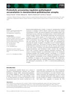
Figure 1 gives the in-domain learning curve.
With fewer training examples, the systems with
N-GM features strongly outperform the LEX-only
system. Note that with tens of thousands of test

5
In this notation, capital letters (and regular expressions)
are matched against tags while a
1
and a
2
match words.
60
65
70
75
80
85
90
95
100
1e51e41e3100
Accuracy (%)
Number of training examples
N-GM+LEX
N-GM
LEX
Figure 1: In-domain learning curve of adjective
ordering classifiers on BNC.
60
65
70
75
80
85

90
95
100
1e51e41e3100
Accuracy (%)
Number of training examples
N-GM+LEX
N-GM
LEX
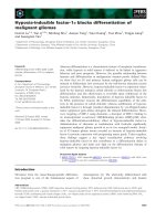
Figure 2: Out-of-domain learning curve of adjec-
tive ordering classifiers on Gutenberg.
examples, all differences are highly significant.
Out-of-domain, LEX’s accuracy drops a shock-
ing 23% on Gutenberg and 19% on Medline (Ta-
ble 1). Malouf (2000)’s system fares even worse.
The overlap between training and test pairs helps
explain. While 59% of the BNC test pairs were
seen in the training corpus, only 25% of Gutenberg
and 18% of Medline pairs were seen in training.
While other ordering models have also achieved
“very poor results” out-of-domain (Mitchell,
2009), we expected our expanded set of LEX fea-
tures to provide good generalization on new data.
Instead, LEX is very unreliable on new domains.
N-GM features do not rely on specific pairs in
training data, and thus remain fairly robust cross-
domain. Across the three test sets, 84-89% of
examples had the correct ordering appear at least
once on the web. On new domains, the learned
N-GM system maintains an advantage over the un-

supervised c(a
1
, a
2
) vs. c(a
2
, a
1
), but the differ-
ence is reduced. Note that training with 10-fold
868
cross validation, the N-GM system can achieve up
to 87.5% on Gutenberg (90.0% for N-GM + LEX).
The learning curve showing performance on
Gutenberg (but still training on BNC) is particu-
larly instructive (Figure 2, performance on Med-
line is very similar). The LEX system performs
much worse than the web-based models across
all training sizes. For our top in-domain sys-
tem, N-GM + LEX, as you add more labeled ex-
amples, performance begins decreasing out-of-
domain. The system disregards the robust N-gram
counts as it is more and more confident in the LEX
features, and it suffers the consequences.
4 Context-Sensitive Spelling Correction
We now turn to the generation problem of context-
sensitive spelling correction. For every occurrence
of a word in a pre-defined set of confusable words
(like peace and piece), the system must select the
most likely word from the set, flagging possible

usage errors when the predicted word disagrees
with the original. Contextual spell checkers are
one of the most widely used NLP technologies,
reaching millions of users via compressed N-gram
models in Microsoft Office (Church et al., 2007).
Our in-domain examples are from the New York
Times (NYT) portion of Gigaword, from Bergsma
et al. (2009). They include the 5 confusion sets
where accuracy was below 90% in Golding and
Roth (1999). There are 100K training, 10K devel-
opment, and 10K test examples for each confusion
set. Our results are averages across confusion sets.
Out-of-domain examples are again drawn from
Gutenberg and Medline. We extract all instances
of words that are in one of our confusion sets,
along with surrounding context. By assuming the
extracted instances represent correct usage, we la-
bel 7.8K and 56K out-of-domain test examples for
Gutenberg and Medline, respectively.
We test three unsupervised systems: 1) Lapata
and Keller (2005) use one token of context on the
left and one on the right, and output the candidate
from the confusion set that occurs most frequently
in this pattern. 2) Bergsma et al. (2009) measure
the frequency of the candidates in all the 3-to-5-
gram patterns that span the confusable word. For
each candidate, they sum the log-counts of all pat-
terns filled with the candidate, and output the can-
didate with the highest total. 3) The baseline pre-
dicts the most frequent member of each confusion

set, based on frequencies in the NYT training data.
System
IN O1 O2
Baseline 66.9 44.6 60.6
Lapata and Keller (2005)
88.4 78.0 87.4
Bergsma et al. (2009)
94.8 87.7 94.2
SVM with N-GM features
95.7 92.1 93.9
SVM with LEX features
95.2 85.8 91.0
SVM with N-GM + LEX
96.5 91.9 94.8
Table 2: Spelling correction accuracy (%). SVM
trained on NYT, tested on NYT (IN) and out-of-
domain Gutenberg (O1) and Medline (O2).
70
75
80
85
90
95
100
1e51e41e3100
Accuracy (%)
Number of training examples
N-GM+LEX
N-GM
LEX

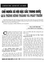
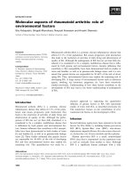
Figure 3: In-domain learning curve of spelling
correction classifiers on NYT.
4.1 Supervised Spelling Correction
Our LEX features are typical disambiguation fea-
tures that flag specific aspects of the context. We
have features for the words at all positions in
a 9-word window (called collocation features by
Golding and Roth (1999)), plus indicators for a
particular word preceding or following the con-
fusable word. We also include indicators for all
N-grams, and their position, in a 9-word window.
For N-GM count features, we follow Bergsma
et al. (2009). We include the log-counts of all
N-grams that span the confusable word, with each
word in the confusion set filling the N-gram pat-
tern. These features do not use part-of-speech.
Following Bergsma et al. (2009), we get N-gram
counts using the original Google N-gram Corpus.
While neither our LEX nor N-GM features are
novel on their own, they have, perhaps surpris-
ingly, not yet been evaluated in a single model.
4.2 Spelling Correction Results
The N-GM features outperform the LEX features,
95.7% vs. 95.2% (Table 2). Together, they
achieve a very strong 96.5% in-domain accuracy.
869
This is 2% higher than the best unsupervised ap-
proach (Bergsma et al., 2009). Web-based models
again perform well across a range of training data
sizes (Figure 3).

The error rate of LEX nearly triples on Guten-
berg and almost doubles on Medline (Table 2). Re-
moving N-GM features from the N-GM + LEX sys-
tem, errors increase around 75% on both Guten-
berg and Medline. The LEX features provide no
help to the combined system on Gutenberg, while
they do help significantly on Medline. Note the
learning curves for N-GM+LEX on Gutenberg and
Medline (not shown) do not display the decrease
that we observed in adjective ordering (Figure 2).
Both the baseline and LEX perform poorly on
Gutenberg. The baseline predicts the majority
class from NYT, but it’s not always the majority
class in Gutenberg. For example, while in NYT
site occurs 87% of the time for the (cite, sight,
site) confusion set, sight occurs 90% of the time in
Gutenberg. The LEX classifier exploits this bias as
it is regularized toward a more economical model,
but the bias does not transfer to the new domain.
5 Noun Compound Bracketing
About 70% of web queries are noun phrases (Barr
et al., 2008) and methods that can reliably parse
these phrases are of great interest in NLP. For
example, a web query for zebra hair straightener
should be bracketed as (zebra (hair straightener)),
a stylish hair straightener with zebra print, rather
than ((zebra hair) straightener), a useless product
since the fur of zebras is already quite straight.
The noun compound (NC) bracketing task is
usually cast as a decision whether a 3-word NC

has a left or right bracketing. Most approaches are
unsupervised, using a large corpus to compare the
statistical association between word pairs in the
NC. The adjacency model (Marcus, 1980) pro-
poses a left bracketing if the association between
words one and two is higher than between two
and three. The dependency model (Lauer, 1995a)
compares one-two vs. one-three. We include de-
pendency model results using PMI as the associ-
ation measure; results were lower with the adja-
cency model.
As in-domain data, we use Vadas and Curran
(2007a)’s Wall-Street Journal (WSJ) data, an ex-
tension of the Treebank (which originally left NPs
flat). We extract all sequences of three consec-
utive common nouns, generating 1983 examples
System
IN O1 O2
Baseline 70.5 66.8 84.1
Dependency model
74.7 82.8 84.4
SVM with N-GM features
89.5 81.6 86.2
SVM with LEX features
81.1 70.9 79.0
SVM with N-GM + LEX
91.6 81.6 87.4
Table 3: NC-bracketing accuracy (%). SVM
trained on WSJ, tested on WSJ (IN) and out-of-
domain Grolier (O1) and Medline (O2).

60
65
70
75
80
85
90
95
100
1e310010
Accuracy (%)
Number of labeled examples
N-GM+LEX
N-GM
LEX
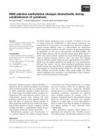
Figure 4: In-domain NC-bracketer learning curve
from sections 0-22 of the Treebank as training, 72
from section 24 for development and 95 from sec-
tion 23 as a test set. As out-of-domain data, we
use 244 NCs from Grolier Encyclopedia (Lauer,
1995a) and 429 NCs from Medline (Nakov, 2007).
The majority class baseline is left-bracketing.
5.1 Supervised Noun Bracketing
Our LEX features indicate the specific noun at
each position in the compound, plus the three pairs
of nouns and the full noun triple. We also add fea-
tures for the capitalization pattern of the sequence.
N-GM features give the log-count of all subsets
of the compound. Counts are from Google V2.
Following Nakov and Hearst (2005), we also in-

clude counts of noun pairs collapsed into a single
token; if a pair occurs often on the web as a single
unit, it strongly indicates the pair is a constituent.
Vadas and Curran (2007a) use simpler features,
e.g. they do not use collapsed pair counts. They
achieve 89.9% in-domain on WSJ and 80.7% on
Grolier. Vadas and Curran (2007b) use compara-
ble features to ours, but do not test out-of-domain.
5.2 Noun Compound Bracketing Results
N-GM systems perform much better on this task
(Table 3). N-GM+LEX is statistically significantly
870
better than LEX on all sets. In-domain, errors
more than double without N-GM features. LEX
performs poorly here because there are far fewer
training examples. The learning curve (Figure 4)
looks much like earlier in-domain curves (Fig-
ures 1 and 3), but truncated before LEX becomes
competitive. The absence of a sufficient amount of
labeled data explains why NC-bracketing is gen-
erally regarded as a task where corpus counts are
crucial.
All web-based models (including the depen-
dency model) exceed 81.5% on Grolier, which
is the level of human agreement (Lauer, 1995b).
N-GM + LEX is highest on Medline, and close
to the 88% human agreement (Nakov and Hearst,
2005). Out-of-domain, the LEX approach per-
forms very poorly, close to or below the base-
line accuracy. With little training data and cross-

domain usage, N-gram features are essential.
6 Verb Part-of-Speech Disambiguation
Our final task is POS-tagging. We focus on one
frequent and difficult tagging decision: the distinc-
tion between a past-tense verb (VBD) and a past
participle (VBN). For example, in the troops sta-
tioned in Iraq, the verb stationed is a VBN; troops
is the head of the phrase. On the other hand, for
the troops vacationed in Iraq, the verb vacationed
is a VBD and also the head. Some verbs make the
distinction explicit (eat has VBD ate, VBN eaten),
but most require context for resolution.
Conflating VBN/VBD is damaging because it af-
fects downstream parsers and semantic role la-
belers. The task is difficult because nearby POS
tags can be identical in both cases. When the
verb follows a noun, tag assignment can hinge on
world-knowledge, i.e., the global lexical relation
between the noun and verb (E.g., troops tends to
be the object of stationed but the subject of vaca-
tioned).
6
Web-scale N-gram data might help im-
prove the VBN/VBD distinction by providing rela-
tional evidence, even if the verb, noun, or verb-
noun pair were not observed in training data.
We extract nouns followed by a VBN/VBD in the
WSJ portion of the Treebank (Marcus et al., 1993),
getting 23K training, 1091 development and 1130
test examples from sections 2-22, 24, and 23, re-

spectively. For out-of-domain data, we get 21K
6
HMM-style taggers, like the fast TnT tagger used on our
web corpus, do not use bilexical features, and so perform es-
pecially poorly on these cases. One motivation for our work
was to develop a fast post-processor to fix VBN/VBD errors.
examples from the Brown portion of the Treebank
and 6296 examples from tagged Medline abstracts
in the PennBioIE corpus (Kulick et al., 2004).
The majority class baseline is to choose VBD.
6.1 Supervised Verb Disambiguation
There are two orthogonal sources of information
for predicting VBN/VBD: 1) the noun-verb pair,
and 2) the context around the pair. Both N-GM
and LEX features encode both these sources.
6.1.1 LEX features
For 1), we use indicators for the noun and verb,
the noun-verb pair, whether the verb is on an in-
house list of said-verb (like warned, announced,
etc.), whether the noun is capitalized and whether
it’s upper-case. Note that in training data, 97.3%
of capitalized nouns are followed by a VBD and
98.5% of said-verbs are VBDs. For 2), we provide
indicator features for the words before the noun
and after the verb.
6.1.2 N-GM features
For 1), we characterize a noun-verb relation via
features for the pair’s distribution in Google V2.
Characterizing a word by its distribution has a
long history in NLP; we apply similar techniques

to relations, like Turney (2006), but with a larger
corpus and richer annotations. We extract the 20
most-frequent N-grams that contain both the noun
and the verb in the pair. For each of these, we con-
vert the tokens to POS-tags, except for tokens that
are among the most frequent 100 unigrams in our
corpus, which we include in word form. We mask
the noun of interest as N and the verb of interest
as V. This converted N-gram is the feature label.
The value is the pattern’s log-count. A high count
for patterns like (N that V), (N have V) suggests
the relation is a VBD, while patterns (N that were
V), (N V by), (V some N) indicate a VBN. As al-
ways, the classifier learns the association between
patterns and classes.
For 2), we use counts for the verb’s context co-
occurring with a VBD or VBN tag. E.g., we see
whether VBD cases like troops ate or VBN cases
like troops eaten are more frequent. Although our
corpus contains many VBN/VBD errors, we hope
the errors are random enough for aggregate counts
to be useful. The context is an N-gram spanning
the VBN/VBD. We have log-count features for all
five such N-grams in the (previous-word, noun,
verb, next-word) quadruple. The log-count is in-
871
System IN O1 O2
Baseline 89.2 85.2 79.6
ContextSum
92.5 91.1 90.4

SVM with N-GM features
96.1 93.4 93.8
SVM with LEX features
95.8 93.4 93.0
SVM with N-GM + LEX
96.4 93.5 94.0
Table 4: Verb-POS-disambiguation accuracy (%)
trained on WSJ, tested on WSJ (IN) and out-of-
domain Brown (O1) and Medline (O2).
80
85
90
95
100
1e41e3100
Accuracy (%)
Number of training examples
N-GM (N,V+context)
LEX (N,V+context)
N-GM (N,V)
LEX (N,V)
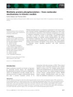
Figure 5: Out-of-domain learning curve of verb
disambiguation classifiers on Medline.
dexed by the position and length of the N-gram.
We include separate count features for contexts
matching the specific noun and for when the noun
token can match any word tagged as a noun.
ContextSum: We use these context counts in an
unsupervised system, ContextSum. Analogously
to Bergsma et al. (2009), we separately sum the

log-counts for all contexts filled with VBD and
then VBN, outputting the tag with the higher total.
6.2 Verb POS Disambiguation Results
As in all tasks, N-GM+LEX has the best in-domain
accuracy (96.4%, Table 4). Out-of-domain, when
N-grams are excluded, errors only increase around
14% on Medline and 2% on Brown (the differ-
ences are not statistically significant). Why? Fig-
ure 5, the learning curve for performance on Med-
line, suggests some reasons. We omit N-GM+LEX
from Figure 5 as it closely follows N-GM.
Recall that we grouped the features into two
views: 1) noun-verb (N,V) and 2) context. If we
use just (N,V) features, we do see a large drop out-
of-domain: LEX (N,V) lags N-GM (N,V) even us-
ing all the training examples. The same is true us-
ing only context features (not shown). Using both
views, the results are closer: 93.8% for N-GM and
93.0% for LEX. With two views of an example,
LEX is more likely to have domain-neutral fea-
tures to draw on. Data sparsity is reduced.
Also, the Treebank provides an atypical num-
ber of labeled examples for analysis tasks. In a
more typical situation with less labeled examples,
N-GM strongly dominates LEX, even when two
views are used. E.g., with 2285 training exam-
ples, N-GM+LEX is statistically significantly bet-
ter than LEX on both out-of-domain sets.
All systems, however, perform log-linearly with
training size. In other tasks we only had a handful

of N-GM features; here there are 21K features for
the distributional patterns of N,V pairs. Reducing
this feature space by pruning or performing trans-
formations may improve accuracy in and out-of-
domain.
7 Discussion and Future Work
Of all classifiers, LEX performs worst on all cross-
domain tasks. Clearly, many of the regularities
that a typical classifier exploits in one domain do
not transfer to new genres. N-GM features, how-
ever, do not depend directly on training examples,
and thus work better cross-domain. Of course, us-
ing web-scale N-grams is not the only way to cre-
ate robust classifiers. Counts from any large auxil-
iary corpus may also help, but web counts should
help more (Lapata and Keller, 2005). Section 6.2
suggests that another way to mitigate domain-
dependence is having multiple feature views.
Banko and Brill (2001) argue “a logical next
step for the research community would be to di-
rect efforts towards increasing the size of anno-
tated training collections.” Assuming we really do
want systems that operate beyond the specific do-
mains on which they are trained, the community
also needs to identify which systems behave as in
Figure 2, where the accuracy of the best in-domain
system actually decreases with more training ex-
amples. Our results suggest better features, such
as web pattern counts, may help more than ex-
panding training data. Also, systems using web-

scale unlabeled data will improve automatically as
the web expands, without annotation effort.
In some sense, using web counts as features
is a form of domain adaptation: adapting a web
model to the training domain. How do we ensure
these features are adapted well and not used in
domain-specific ways (especially with many fea-
tures to adapt, as in Section 6)? One option may
872
be to regularize the classifier specifically for out-
of-domain accuracy. We found that adjusting the
SVM misclassification penalty (for more regular-
ization) can help or hurt out-of-domain. Other
regularizations are possible. In each task, there
are domain-neutral unsupervised approaches. We
could encode these systems as linear classifiers
with corresponding weights. Rather than a typical
SVM that minimizes the weight-norm ||w|| (plus
the slacks), we could regularize toward domain-
neutral weights. This regularization could be opti-
mized on creative splits of the training data.
8 Conclusion
We presented results on tasks spanning a range of
NLP research: generation, disambiguation, pars-
ing and tagging. Using web-scale N-gram data
improves accuracy on each task. When less train-
ing data is used, or when the system is used on a
different domain, N-gram features greatly improve
performance. Since most supervised NLP systems
do not use web-scale counts, further cross-domain

evaluation may reveal some very brittle systems.
Continued effort in new domains should be a pri-
ority for the community going forward.
Acknowledgments
We gratefully acknowledge the Center for Lan-
guage and Speech Processing at Johns Hopkins
University for hosting the workshop at which part
of this research was conducted.
References
Nir Ailon and Mehryar Mohri. 2008. An efficient re-
duction of ranking to classification. In COLT.
Michele Banko and Eric Brill. 2001. Scaling to very
very large corpora for natural language disambigua-
tion. In ACL.
Cory Barr, Rosie Jones, and Moira Regelson. 2008.
The linguistic structure of English web-search
queries. In EMNLP.
Shane Bergsma, Dekang Lin, and Randy Goebel.
2009. Web-scale N-gram models for lexical disam-
biguation. In IJCAI.
John Blitzer, Mark Dredze, and Fernando Pereira.
2007. Biographies, bollywood, boom-boxes and
blenders: Domain adaptation for sentiment classi-
fication. In ACL.
Thorsten Brants and Alex Franz. 2006. The Google
Web 1T 5-gram Corpus Version 1.1. LDC2006T13.
Thorsten Brants, Ashok C. Popat, Peng Xu, Franz J.
Och, and Jeffrey Dean. 2007. Large language mod-
els in machine translation. In EMNLP.
Thorsten Brants. 2000. TnT – a statistical part-of-

speech tagger. In ANLP.
Andrew Carlson, Tom M. Mitchell, and Ian Fette.
2008. Data analysis project: Leveraging massive
textual corpora using n-gram statistics. Technial Re-
port CMU-ML-08-107.
Kenneth Church, Ted Hart, and Jianfeng Gao. 2007.
Compressing trigram language models with Golomb
coding. In EMNLP-CoNLL.
Hal Daum´e III. 2007. Frustratingly easy domain adap-
tation. In ACL.
Rong-En Fan, Kai-Wei Chang, Cho-Jui Hsieh, Xiang-
Rui Wang, and Chih-Jen Lin. 2008. LIBLINEAR:
A library for large linear classification. Journal of
Machine Learning Research, 9.
Dan Gildea. 2001. Corpus variation and parser perfor-
mance. In EMNLP.
Andrew R. Golding and Dan Roth. 1999. A Winnow-
based approach to context-sensitive spelling correc-
tion. Machine Learning, 34(1-3):107–130.
Thorsten Joachims. 2002. Optimizing search engines
using clickthrough data. In KDD.
Frank Keller and Mirella Lapata. 2003. Using the web
to obtain frequencies for unseen bigrams. Computa-
tional Linguistics, 29(3):459–484.
Adam Kilgarriff and Gregory Grefenstette. 2003. In-
troduction to the special issue on the Web as corpus.
Computational Linguistics, 29(3):333–347.
Seth Kulick, Ann Bies, Mark Liberman, Mark Mandel,
Ryan McDonald, Martha Palmer, Andrew Schein,
Lyle Ungar, Scott Winters, and Pete White. 2004.

Integrated annotation for biomedical information ex-
traction. In BioLINK 2004: Linking Biological Lit-
erature, Ontologies and Databases.
Mirella Lapata and Frank Keller. 2005. Web-based
models for natural language processing. ACM
Transactions on Speech and Language Processing,
2(1):1–31.
Mark Lauer. 1995a. Corpus statistics meet the noun
compound: Some empirical results. In ACL.
Mark Lauer. 1995b. Designing Statistical Language
Learners: Experiments on Compound Nouns. Ph.D.
thesis, Macquarie University.
Dekang Lin, Kenneth Church, Heng Ji, Satoshi Sekine,
David Yarowsky, Shane Bergsma, Kailash Patil,
Emily Pitler, Rachel Lathbury, Vikram Rao, Kapil
Dalwani, and Sushant Narsale. 2010. New tools for
web-scale N-grams. In LREC.
873
Robert Malouf. 2000. The order of prenominal adjec-
tives in natural language generation. In ACL.
Mitchell P. Marcus, Beatrice Santorini, and Mary
Marcinkiewicz. 1993. Building a large annotated
corpus of English: The Penn Treebank. Computa-
tional Linguistics, 19(2):313–330.
Mitchell P. Marcus. 1980. Theory of Syntactic Recog-
nition for Natural Languages. MIT Press, Cam-
bridge, MA, USA.
David McClosky, Eugene Charniak, and Mark John-
son. 2006. Reranking and self-training for parser
adaptation. In COLING-ACL.

Margaret Mitchell. 2009. Class-based ordering of
prenominal modifiers. In 12th European Workshop
on Natural Language Generation.
Natalia N. Modjeska, Katja Markert, and Malvina Nis-
sim. 2003. Using the Web in machine learning for
other-anaphora resolution. In EMNLP.
Preslav Nakov and Marti Hearst. 2005. Search engine
statistics beyond the n-gram: Application to noun
compound bracketing. In CoNLL.
Preslav Ivanov Nakov. 2007. Using the Web as an Im-
plicit Training Set: Application to Noun Compound
Syntax and Semantics. Ph.D. thesis, University of
California, Berkeley.
Xuan-Hieu Phan. 2006. CRFTagger: CRF English
POS Tagger. crftagger.sourceforge.net.
Laura Rimell and Stephen Clark. 2008. Adapting a
lexicalized-grammar parser to contrasting domains.
In EMNLP.
James Shaw and Vasileios Hatzivassiloglou. 1999. Or-
dering among premodifiers. In ACL.
Yoshimasa Tsuruoka, Yuka Tateishi, Jin-Dong Kim,
Tomoko Ohta, John McNaught, Sophia Ananiadou,
and Jun’ichi Tsujii. 2005. Developing a robust part-
of-speech tagger for biomedical text. In Advances in
Informatics.
Peter D. Turney. 2006. Similarity of semantic rela-
tions. Computational Linguistics, 32(3):379–416.
David Vadas and James R. Curran. 2007a. Adding
noun phrase structure to the Penn Treebank. In ACL.
David Vadas and James R. Curran. 2007b. Large-scale

supervised models for noun phrase bracketing. In
PACLING.
Xiaofeng Yang, Jian Su, and Chew Lim Tan. 2005.
Improving pronoun resolution using statistics-based
semantic compatibility information. In ACL.
874