Condensed phase molecular spectroscopy and photophysics
Bạn đang xem bản rút gọn của tài liệu. Xem và tải ngay bản đầy đủ của tài liệu tại đây (7.43 MB, 332 trang )
CONDENSED-PHASE
MOLECULAR
SPECTROSCOPY AND
PHOTOPHYSICS
CONDENSED-PHASE
MOLECULAR
SPECTROSCOPY AND
PHOTOPHYSICS
ANNE MYERS KELLEY
A JOHN WILEY & SONS, INC., PUBLICATION
www.pdfgrip.com
Copyright © 2013 by John Wiley & Sons, Inc. All rights reserved
Published by John Wiley & Sons, Inc., Hoboken, New Jersey
Published simultaneously in Canada
No part of this publication may be reproduced, stored in a retrieval system, or transmitted in
any form or by any means, electronic, mechanical, photocopying, recording, scanning, or
otherwise, except as permitted under Section 107 or 108 of the 1976 United States Copyright
Act, without either the prior written permission of the Publisher, or authorization through
payment of the appropriate per-copy fee to the Copyright Clearance Center, Inc., 222
Rosewood Drive, Danvers, MA 01923, (978) 750-8400, fax (978) 750-4470, or on the web at
www.copyright.com. Requests to the Publisher for permission should be addressed to the
Permissions Department, John Wiley & Sons, Inc., 111 River Street, Hoboken, NJ 07030, (201)
748-6011, fax (201) 748-6008, or online at />Limit of Liability/Disclaimer of Warranty: While the publisher and author have used their best
efforts in preparing this book, they make no representations or warranties with respect to the
accuracy or completeness of the contents of this book and specifically disclaim any implied
warranties of merchantability or fitness for a particular purpose. No warranty may be created
or extended by sales representatives or written sales materials. The advice and strategies
contained herein may not be suitable for your situation. You should consult with a professional
where appropriate. Neither the publisher nor author shall be liable for any loss of profit or any
other commercial damages, including but not limited to special, incidental, consequential, or
other damages.
For general information on our other products and services or for technical support, please
contact our Customer Care Department within the United States at (800) 762-2974, outside the
United States at (317) 572-3993 or fax (317) 572-4002.
Wiley also publishes its books in a variety of electronic formats. Some content that appears in
print may not be available in electronic formats. For more information about Wiley products,
visit our web site at www.wiley.com.
Library of Congress Cataloging-in-Publication Data is available
ISBN 9780470946701
Printed in the United States of America
10 9 8 7 6 5 4 3 2 1
www.pdfgrip.com
CONTENTS
PREFACE
xi
1 REVIEW OF TIME-INDEPENDENT QUANTUM MECHANICS
1
1.1 States, Operators, and Representations / 1
1.2 Eigenvalue Problems and the Schrödinger Equation / 4
1.3 Expectation Values, Uncertainty Relations / 6
1.4 The Particle in a Box / 7
1.5 Harmonic Oscillator / 9
1.6 The Hydrogen Atom and Angular Momentum / 12
1.7 Approximation Methods / 15
1.8 Electron Spin / 18
1.9 The Born–Oppenheimer Approximation / 22
1.10 Molecular Orbitals / 22
1.11 Energies and Time Scales; Separation of Motions / 25
Further Reading / 26
Problems / 27
2 ELECTROMAGNETIC RADIATION
2.1
2.2
2.3
31
Classical Description of Light / 31
Quantum Mechanical Description of Light / 35
Fourier Transform Relationships Between Time and
Frequency / 38
v
www.pdfgrip.com
vi
CONTENTS
2.4 Blackbody Radiation / 40
2.5 Light Sources for Spectroscopy / 42
References and Further Reading / 44
Problems / 44
3 RADIATION–MATTER INTERACTIONS
47
3.1 The Time-Dependent Schrödinger Equation / 47
3.2 Time-Dependent Perturbation Theory / 50
3.3 Interaction of Matter with the Classical Radiation Field / 54
3.4 Interaction of Matter with the Quantized Radiation Field / 59
References and Further Reading / 63
Problems / 64
4 ABSORPTION AND EMISSION OF LIGHT
67
4.1 Einstein Coefficients for Absorption and Emission / 67
4.2 Other Measures of Absorption Strength / 69
4.3 Radiative Lifetimes / 72
4.4 Oscillator Strengths / 73
4.5 Local Fields / 73
Further Reading / 74
Problems / 75
5 SYSTEM–BATH INTERACTIONS
79
5.1 Phenomenological Treatment of Relaxation and Lineshapes / 79
5.2 The Density Matrix / 86
5.3 Density Matrix Methods in Spectroscopy / 90
5.4 Exact Density Matrix Solution for a Two-Level System / 95
References and Further Reading / 98
Problems / 98
6 SYMMETRY CONSIDERATIONS
6.1
6.2
6.3
Qualitative Aspects of Molecular Symmetry / 103
Introductory Group Theory / 104
Finding the Symmetries of Vibrational Modes of a Certain
Type / 109
6.4 Finding the Symmetries of All Vibrational Modes / 111
Further Reading / 113
Problems / 113
www.pdfgrip.com
103
CONTENTS
7 MOLECULAR VIBRATIONS AND INFRARED
SPECTROSCOPY
vii
115
7.1 Vibrational Transitions / 115
7.2 Diatomic Vibrations / 117
7.3 Anharmonicity / 118
7.4 Polyatomic Molecular Vibrations: Normal Modes / 121
7.5 Symmetry Considerations / 127
7.6 Isotopic Shifts / 130
7.7 Solvent Effects on Vibrational Spectra / 130
References and Further Reading / 135
Problems / 135
8 ELECTRONIC SPECTROSCOPY
139
8.1 Electronic Transitions / 139
8.2 Spin and Orbital Selection Rules / 141
8.3 Spin–Orbit Coupling / 143
8.4 Vibronic Structure / 143
8.5 Vibronic Coupling / 148
8.6 The Jahn–Teller Effect / 151
8.7 Considerations in Large Molecules / 152
8.8 Solvent Effects on Electronic Spectra / 154
Further Reading / 159
Problems / 160
9 PHOTOPHYSICAL PROCESSES
163
9.1 Jablonski Diagrams / 163
9.2 Quantum Yields and Lifetimes / 166
9.3 Fermi’s Golden Rule for Radiationless Transitions / 167
9.4 Internal Conversion and Intersystem Crossing / 167
9.5 Intramolecular Vibrational Redistribution / 173
9.6 Energy Transfer / 179
9.7 Polarization and Molecular Reorientation in Solution / 182
References and Further Reading / 186
Problems / 186
10 LIGHT SCATTERING
191
10.1 Rayleigh Scattering from Particles / 191
10.2 Classical Treatment of Molecular Raman and Rayleigh
Scattering / 193
www.pdfgrip.com
viii
CONTENTS
10.3 Quantum Mechanical Treatment of Molecular Raman and
Rayleigh Scattering / 195
10.4 Nonresonant Raman Scattering / 204
10.5 Symmetry Considerations and Depolarization Ratios in Raman
Scattering / 206
10.6 Resonance Raman Spectroscopy / 207
References and Further Reading / 211
Problems / 211
11 NONLINEAR AND PUMP–PROBE SPECTROSCOPIES
215
11.1 Linear and Nonlinear Susceptibilities / 215
11.2 Multiphoton Absorption / 216
11.3 Pump–Probe Spectroscopy: Transient Absorption and Stimulated
Emission / 219
11.4 Vibrational Oscillations and Impulsive Stimulated
Scattering / 225
11.5 Second Harmonic and Sum Frequency Generation / 227
11.6 Four-Wave Mixing / 232
11.7 Photon Echoes / 232
References and Further Reading / 234
Problems / 234
12 ELECTRON TRANSFER PROCESSES
239
12.1 Charge–Transfer Transitions / 239
12.2 Marcus Theory / 243
12.3 Spectroscopy of Anions and Cations / 247
References and Further Reading / 248
Problems / 248
13 COLLECTIONS OF MOLECULES
251
13.1 Van der Waals Molecules / 251
13.2 Dimers and Aggregates / 252
13.3 Localized and Delocalized Excited States / 253
13.4 Conjugated Polymers / 256
References / 259
Problems / 259
14 METALS AND PLASMONS
14.1 Dielectric Function of a Metal / 263
14.2 Plasmons / 266
www.pdfgrip.com
263
CONTENTS
ix
14.3 Spectroscopy of Metal Nanoparticles / 268
14.4 Surface-Enhanced Raman and Fluorescence / 270
References and Further Reading / 274
Problems / 275
15 CRYSTALS
277
15.1 Crystal Lattices / 277
15.2 Phonons in Crystals / 281
15.3 Infrared and Raman Spectra / 284
15.4 Phonons in Nanocrystals / 286
References and Further Reading / 287
Problems / 287
16 ELECTRONIC SPECTROSCOPY OF SEMICONDUCTORS
291
16.1 Band Structure / 291
16.2 Direct and Indirect Transitions / 296
16.3 Excitons / 296
16.4 Defects / 298
16.5 Semiconductor Nanocrystals / 298
Further Reading / 302
Problems / 302
APPENDICES
A PHYSICAL CONSTANTS, UNIT SYSTEMS,
AND CONVERSION FACTORS
B MISCELLANEOUS MATHEMATICS REVIEW
C MATRICES AND DETERMINANTS
D CHARACTER TABLES FOR SOME COMMON
POINT GROUPS
E FOURIER TRANSFORMS
317
321
INDEX
323
www.pdfgrip.com
305
309
313
PREFACE
Faculty members teaching advanced or graduate level courses in their specialty tend to have well-defined ideas about how such courses should be
taught—what material should be covered and in what depth, how the topics
should be organized, and what “point of view” should be adopted. There are
probably as many different ideas about how to teach any graduate course as
there are individuals doing the teaching. It is therefore no surprise that many
faculty cannot find any single textbook that truly meets their needs for any
given course. Most simply accept this situation, and either choose the book
they like best (or dislike least) and supplement it with other textbooks and/or
notes, or adopt no primary text at all. A few become sufficiently unhappy with
the lack of a suitable text that they decide to write one themselves. This book
is the outcome of such a decision.
Most chemistry departments offer a course in molecular spectroscopy for
graduate students and advanced undergraduates. Some very good textbooks
have been written for traditional molecular spectroscopy courses, but my
favorite and that of many others, Walter Struve’s Fundamentals of Molecular
Spectroscopy, is now out of print. Furthermore, most traditional textbooks
focus on high-resolution spectroscopy of small molecules in the gas phase, and
topics such as rotational spectroscopy and rotation–vibration interactions that
are not the most relevant to much current research in chemistry programs. A
great deal of modern research involves the interaction of radiation with condensed-phase systems, such as molecules in liquids, solids, and more complex
media, molecular aggregates, metals and semiconductors, and their composites.
There is a need for a graduate-level textbook that covers the basics of traditional molecular spectroscopy but takes a predominantly condensed-phase
xi
www.pdfgrip.com
xii
Preface
perspective and also addresses optical processes in extended systems, such as
metals, semiconductors, and conducting polymers.
This book aims to provide a treatment of radiation–matter interactions that
is useful for molecules in condensed phases, as well as supramolecular structures and nanostructures. The book is written at a level appropriate for
advanced undergraduates or beginning graduate students in physical or materials chemistry. Much of the organization and topic selection is similar to that
of a traditional graduate-level molecular spectroscopy text, but atomic spectroscopy, rotational spectroscopy, and other topics relevant mainly to gasphase systems are omitted entirely, and there is much more emphasis on the
molecule–environment interactions that strongly influence spectra in condensed phases. Additions often not found in molecular spectroscopy texts
include the spectroscopy and photophysics of molecular aggregates and
molecular solids and of metals and semiconductors, with particular emphasis
on nanoscale size regimes. Spin-resonance methods (e.g., NMR and ESR) are
not covered, nor are x-ray or electron spectroscopies. Experimental techniques
are addressed only to the extent needed to understand spectroscopic data.
Chapters 1 through 10 address spectroscopic fundamentals that should
probably be included in any spectroscopy course or in prerequisite courses.
Chapters 11 through 16 are less fundamental, and some will probably need to
be omitted in a one-semester spectroscopy course, and certainly in a onequarter course. The instructor may choose to omit all of these remaining
chapters or may pick and choose among them to tailor the course. It is assumed
that students using this book have already taken a course in basic quantum
mechanics and many instructors may choose to omit explicit coverage of
Chapter 1, but it is included for review and reference as it is essential to understanding what comes later. Instructors may also wish to omit Chapter 6 if it is
assumed that students have been introduced to group theory in undergraduate
inorganic chemistry or quantum chemistry courses.
Textbooks of this type inevitably reflect the experiences and biases of their
authors, and this one is no exception. Group theory is discussed in less depth
and is used less extensively than in most spectroscopy textbooks. Raman and
resonance Raman scattering are developed in considerable detail, while most
other multiphoton spectroscopies are treated only at a rather superficial level.
Spectroscopies that involve circularly polarized light, such as circular dichroism, are ignored completely. These all represent choices made in an effort to
keep this book a reasonable length while trying to optimize its usefulness for
a wide range of students. Only time will tell how well I have succeeded.
The general structure and emphasis of this book developed largely from
discussions with David Kelley, whose encouragement pushed me over the edge
from thinking about writing a book to actually doing it. He would not have
written the same book I did, but his input proved valuable at many stages. I
would also like to acknowledge the graduate students in my Spring 2012
Molecular Spectroscopy course (Gary Abel, Joshua Baker, Ke Gong, Cheetar
Lee, and Xiao Li) for patiently pointing out numerous typographical errors,
www.pdfgrip.com
Preface
xiii
notational inconsistencies, and confusing explanations present in the first draft
of this book. Their input was very helpful in bringing this project to its
conclusion.
Anne Myers Kelley
Merced, CA
May 2012
www.pdfgrip.com
CHAPTER 1
REVIEW OF TIME-INDEPENDENT
QUANTUM MECHANICS
While some spectroscopic observations can be understood using purely classical concepts, most molecular spectroscopy experiments probe explicitly
quantum mechanical properties. It is assumed that students using this text have
already taken a course in basic quantum mechanics, but it is also recognized
that there are likely to be some holes in the preparation of most students and
that all can benefit from a brief review. As this is not a quantum mechanics
textbook, many results in this chapter are given without proof and with
minimal explanation. Students seeking a deeper treatment are encouraged to
consult the references given at the end of this chapter.
This chapter, like most introductory quantum chemistry courses, focuses on
solutions of the time-independent Schrödinger equation. Because of the
importance of time-dependent quantum mechanics in spectroscopy, that topic
is discussed further in Chapter 2.
1.1. STATES, OPERATORS, AND REPRESENTATIONS
A quantum mechanical system consisting of N particles (usually electrons and/
or nuclei) is represented most generally by a state function or state vector Ψ.
The state vector contains, in principle, all information about the quantum
mechanical system.
Condensed-Phase Molecular Spectroscopy and Photophysics, First Edition. Anne Myers Kelley.
© 2013 John Wiley & Sons, Inc. Published 2013 by John Wiley & Sons, Inc.
1
www.pdfgrip.com
2
Review of Time-Independent Quantum Mechanics
In order to be useful, state vectors have to be expressed in some basis. In
the most commonly used position basis, the state vector is called the wavefunction, written as Ψ(r1, r2, . . . rN), where ri is the position in space of particle i.
The position r may be expressed in Cartesian coordinates (x, y, z), spherical
polar coordinates (r, θ, φ), or some other coordinate system. Wavefunctions
may alternatively be expressed in the momentum basis, Ψ(p1, p2, . . . pN), where
pi is the momentum of particle i. Some state vectors cannot be expressed as a
function of position, such as those representing the spin of an electron. But
there’s always a state function that describes the system, even if it’s not a
“function” of ordinary spatial coordinates.
The wavefunction itself, also known as the probability amplitude, is not
directly measurable and has no simple physical interpretation. However, the
quantity |Ψ(r1, r2, . . . rN)|2 dr1dr2 . . . drN gives the probability that particle 1 is
in some infinitesimal volume element around r1, and so on. Integration over a
finite volume then gives the probability that the system is found within that
volume. A “legal” wavefunction has to be single valued, continuous, differentiable, and normalizable.
The scalar product or inner product of two wavefunctions Ψ and Φ is given
by ∫Ψ*Φ, where the asterisk means complex conjugation and the integration
is performed over all of the coordinates of all the particles. The inner product
is not a function but a number, generally a complex number if the wavefunctions are complex. In Dirac notation, this inner product is denoted 〈Ψ|Φ〉. The
absolute square of the inner product, |〈Ψ|Φ〉|2, gives the probability (a real
number) that a system in state Ψ is also in state Φ. If 〈Ψ|Φ〉 = 0, then Ψ and Φ
are said to be orthogonal. Reversing the order in Dirac notation corresponds
to taking the complex conjugate of the inner product: 〈Φ|Ψ〉 = ∫Φ*Ψ, while
〈Ψ|Φ〉 = ∫Ψ*Φ = (∫Φ*Ψ)*.
The inner product of a wavefunction with itself, 〈Ψ|Ψ〉 = ∫Ψ*Ψ, is always
real and positive. Usually, wavefunctions are chosen to be normalized to
∫Ψ*Ψ = 1. This means that the probability of finding the system somewhere in
space is unity.
The quantities we are used to dealing with in classical mechanics are represented in quantum mechanics by operators. Operators act on wavefunctions
or state vectors to give other wavefunctions or state vectors. Operator A acting
on wavefunction Ψ to give wavefunction Φ is written as AΨ = Φ. The action
of an operator can be as simple as multiplication, although many (not all)
operators involve differentiation.
Quantum mechanical operators are linear, which means that if λ1 and λ2
are numbers (not states or operators), then A(λ1Φ1 + λ2Φ2) = λ1AΦ1 + λ2AΦ2,
and (AB)Φ = A(BΦ) = ABΦ. However, it is not true in general that
ABΦ = BAΦ; the order in which the operators are applied often matters. The
quantity AB − BA is called the commutator of A and B and is symbolized
[A, B], and it is zero for some pairs of operators but not for all. Most of what
is “interesting” (i.e., nonclassical) about quantum mechanical systems arises
from the noncommutation of certain operators.
www.pdfgrip.com
States, Operators, and Representations
3
A representation is a set of basis vectors, which may be discrete (finite or
infinite) or continuous. An example of a finite discrete basis is the eigenstates
of the z-component of spin for a spin-1/2 particle (two states, usually called α
and β). An example of a discrete infinite basis is the set of eigenstates of a
one-dimensional harmonic oscillator, {ψv}, where v must be an integer but can
go from 0 to ∞. An example of a continuous basis is the position basis {r},
where r can take on any real value. To be a representation, a set of basis vectors
must obey certain extra conditions. One is orthonormality: 〈ui|uj〉 = δij (the
Kronecker delta) for a discrete basis, or 〈wα|wα′〉 = δ(α-α′) (the Dirac delta
function) for a continuous basis. The Kronecker delta is defined by δij = 1 if
i = j, δij = 0 if i ≠ j. The Dirac delta function δ(α-α′) is a hypothetical function
of the variable α that is infinitely sharply peaked around α = α′ and has an
integrated area of unity. Three useful properties of the Dirac delta function
are:
∫
∫
∞
dke ikx = 2πδ( x)
(1.1)
dxf ( x)δ ( x − a) = f (a)
(1.2)
−∞
∞
−∞
δ (ax ) = δ( x) / a ,
(1.3)
where a is a constant.
A set of vectors in a particular state space is a basis if every state in that
space has a unique expansion, such that Ψ = Σiciui (discrete basis) or
Ψ = ∫dαc(α)wα (continuous basis), where the c’s are (complex) numbers. “In
a particular state space” means, for example, that if we want to describe only
the spin state of a system, the basis does not have to include the spatial degrees
of freedom. Or, the states of position in one dimension {x} can be a basis for
a particle in a one-dimensional box, but not a two-dimensional box, which
requires a two-dimensional position basis {(x,y)}. An important property of a
representation is closure:
∑
i
∫
Φ ui ui Ψ = Φ Ψ or dα Φ wα wα Ψ = Φ Ψ .
(1.4)
Representations of states and operators in discrete bases are often conveniently written in matrix form (see Appendix C). A state vector is represented
in a basis by a column vector of numbers:
u1 Ψ
u2 Ψ ,
and its complex conjugate by a row vector: (〈Φ|u1〉〈Φ|u2〉 · · ·). The inner product
is then obtained by the usual rules for matrix multiplication as
www.pdfgrip.com
4
Review of Time-Independent Quantum Mechanics
Φ Ψ = ( Φ u1 Φ u2
u1 Ψ
) u2 Ψ = a number.
An operator is represented by a square matrix having elements Aij = 〈ui|A|uj〉:
u1 A u1
u2 A u1
u1 A u2
u2 A u2
For Hermitian operators, Aji* = Aij. It follows that the diagonal elements must
be real for Hermitian operators, since only then can Aii* = Aii.
The operator expression AΨ = Φ is represented in the {ui} basis as the
matrix equation
u1 A u1
u2 A u1
u1 A u2
u2 A u2
u1 Ψ u1 Φ
u2 Ψ = u2 Φ
1.2. EIGENVALUE PROBLEMS AND THE SCHRÖDINGER EQUATION
The state Ψ is an eigenvector or eigenstate of operator A with eigenvalue λ
if AΨ = λΨ, where λ is a number. That is, operating on Ψ with A just multiplies
Ψ by a constant. The eigenvalue λ is nondegenerate if there is only one eigenstate having that eigenvalue. If more than one distinct state (wavefunctions
that differ from each other by more than just an overall multiplicative constant) has the same eigenvalue, then that eigenvalue is degenerate.
To every observable (measurable quantity) in classical mechanics, there
corresponds a linear, Hermitian operator in quantum mechanics. Since observables correspond to measurable things, this means all observables have only
real eigenvalues. It can be shown from this that eigenfunctions of the same
observable having different eigenvalues are necessarily orthogonal (orthonormal if we require they be normalized).
In Dirac notation, using basis {ui}, the eigenvalue equation is 〈ui|A|Ψ〉 =
λ〈ui|Ψ〉. Inserting closure gives Σj〈ui|A|uj〉〈uj|Ψ〉 = λ〈ui|Ψ〉, or in a shorter form
ΣjAijcj = λci, or in an even more compact form, Σj{Aij − λδij}cj = 0. This is a
system of N equations (one for each i) in N unknowns, which has a nontrivial
solution if and only if the determinant of the coefficients is zero: |A − λ1| = 0,
where 1 is an N × N unit matrix (1’s along the diagonal). So to find the eigenvalues, we need to set up the determinantal equation
A11 − λ
A21
A12
A22 − λ
www.pdfgrip.com
= 0,
Eigenvalue Problems and the Schrödinger Equation
5
and solve for the N roots λ, then find the eigenvector corresponding to each
eigenvalue λ(i) by solving the matrix equation
A11
A21
A12
A22
(i )
c1( i )
c1
c2( i ) = λ ( i ) c2( i )
(see Appendix C).
Any measurement of the observable associated with operator A can give
only those values that are eigenvalues of A. If the system is in an eigenstate
of the operator, then every measurement will yield the same value, the eigenvalue. If the system is not in an eigenstate, different measurements will yield
different values, but each will be one of the eigenvalues.
A particularly important observable is the one associated with the total
energy of the system. This operator is called the Hamiltonian, symbolized H,
the sum of the kinetic and potential energy operators. The eigenstates of the
Hamiltonian are therefore eigenstates of the energy, and the associated eigenvalues represent the only values that can result from any measurement of the
energy of that system.
To find the energy eigenvalues and eigenstates, one must first write down
the appropriate Hamiltonian for the problem at hand, which really amounts
to identifying the potential function in which the particles move, since the
kinetic energy is straightforward. One then solves the eigenvalue problem
Hψn = Enψn, which is the time-independent Schrödinger equation. For most
Hamiltonians, there are many different pairs of wavefunctions ψn and energies
En that can satisfy the equation.
Two observables of particular importance in quantum mechanics are the
position Q and the linear momentum P along the same coordinate (e.g., x and
px). The commutator is [Q, P] = iħ and the action of P in the q representation
is −iħ(∂/∂q). That is, PΨ(q) = −iħ(∂/∂q)Ψ(q), where Ψ(q) is the wavefunction
as a function of the coordinate q. The operator P2 = PP in the q representation is −ħ2(∂2/∂q2).
The Schrödinger equation in the position basis, HΨ(q) = EΨ(q), can therefore be written for a particle moving in only one dimension as
[( p2 / 2m) + V (q)]Ψ(q) = EΨ(q),
(1.5)
−( 2 / 2 m){∂ 2 Ψ(q)/∂q2 } + V (q)Ψ(q) = EΨ(q).
(1.6)
or
ˆ
The position operator in three dimensions is a vector, = xˆ x + yˆ y + zˆz , where x,
ˆ and zˆ are unit vectors along x, y, and z directions. The momentum operator
y,
is also a vector, which in the position basis is
www.pdfgrip.com
6
Review of Time-Independent Quantum Mechanics
p = −i(xˆ ∂ /∂x + yˆ ∂ /∂y + zˆ∂ /∂z) = −i ٌ,
(1.7)
where ∇ is called the del or grad operator. The square of the momentum is
p 2 = p ⋅ p = − 2 (xˆ ∂ /∂x + yˆ ∂ /∂y + zˆ∂ /∂z) ⋅ (xˆ ∂ /∂x + yˆ ∂ /∂y + zˆ∂ /∂z)
= − 2 (∂ 2 / ∂ x 2 + ∂ 2 / ∂ y 2 + ∂ 2 / ∂ z 2 ) = − 2 ∇ 2 ,
(1.8)
where ∇2 is called the Laplacian. Notice that while the momentum is a vector,
the momentum squared is not.
1.3. EXPECTATION VALUES, UNCERTAINTY RELATIONS
When a system is in state Ψ, the mean value or expectation value of observable
A is defined as the average of a large number of measurements. It is given by
〈A〉 = 〈Ψ|A|Ψ〉 = ∫Ψ*AΨ. If Ψ is an eigenfunction of A, then we’ll always
measure the same number, the eigenvalue, for the observable a. If Ψ is not an
eigenfunction of A, then each measurement may yield a different value, but
we can calculate its average with complete certainty from the previous expression. Note that if A involves just multiplication, such as q to some power, we
can just write this as 〈qn〉 = ∫|Ψ(q)|2 qn dq. But if A does something like differentiation, then we have to make sure it operates on Ψ(q) only, not also
Ψ*(q). For example, for momentum, p = −iħ(∂/∂q), we have 〈p〉 = −iħ∫Ψ*(q)
{(∂/∂q)Ψ(q)}dq.
The root-mean-square deviation of the value of operator A in state Ψ is
∆A =
( A − A )2
(1.9a)
that is, ∆A = (A − Aavg )2 . Note that if Ψ is an eigenstate of A, then ΔA = 0,
since every measurement of A gives the same result. An alternative and
sometimes preferable form for ΔA can be written by noting that since 〈A〉 is
a number, 〈(A − 〈A〉)2〉 = 〈A2 − 2A〈A〉 + 〈A〉2〉 = 〈A2〉 − 2〈A〉2 + 〈A〉2 = 〈A2〉 −
〈A〉2. So,
∆A =
A2 − A
2
(1.9b)
is an alternative equivalent form.
The product of the root-mean-square deviations of two operators A and B,
in any state, obeys the relationship
∆A∆B ≥
1
[A, B] .
2
(1.10)
A particularly important example is for the various components of position
and momentum; since [Q, P] = iħ, then ΔQΔP ≥ ħ/2. This is often known as
www.pdfgrip.com
The Particle in a Box
7
the Heisenberg uncertainty relation between position and momentum. The
interpretation is that you cannot simultaneously know both the position and
the momentum along the same direction (e.g., x and px) to arbitrary accuracy;
their uncertainty product, ΔQΔP, has a finite nonzero value. Only for operators
that commute can the uncertainty product vanish (although it is not necessarily
zero in any state). Note that since different components of position and
momentum (e.g., x and py) do commute, their uncertainty product can be zero.
Because commuting observables can have a zero uncertainty product, they
are said to be compatible observables. This means that if [A,B] = 0, and
AΨ = aΨ, (Ψ is an eigenstate of the operator A), then the state given by (BΨ)
is also an eigenstate of A with the same eigenvalue. The result one gets from
a measurement of A is not affected by having previously measured B. One
can have simultaneous eigenstates of A and B. In general, this is not the case
if the operators do not commute.
1.4. THE PARTICLE IN A BOX
The “particle in a box,” in one dimension, refers to a particle of mass m in a
potential defined by V(x) = 0 for 0 ≤ x ≤ a, and V(x) = ∞ everywhere else. In
one dimension, this may be used to model an electron in a delocalized molecular orbital, for example, the pi-electron system of a linear polyene molecule,
conjugated polymer, or porphyrin. In three dimensions, it may be used to
model the electronic states of a semiconductor nanocrystal.
Since the potential energy becomes infinite at the walls, the boundary condition is that the wavefunction must go to zero at both walls. Thus, the relevant
Schrödinger equation becomes (in 1-D)
−( 2 / 2 m)(d 2 /dx 2 )ψ ( x) = Eψ ( x) for 0 ≤ x ≤ a.
(1.11)
The solutions to this equation are
ψ n ( x) = B sin(nπx /a) and En = h2 n2 / 8 ma2
for n = 1, 2, …. (1.12)
The function will be a solution for any value of the constant B. We find B by
requiring that ψn(x) be normalized: that is, the total probability of finding the
a
particle somewhere in space must be unity. This means that ∫ 0 dx ψ n ( x) 2 = 1,
and we find B = 2 / a . These solutions are plotted in Figure 1.1.
The particle in a box in two or three dimensions is a simple extension of
the 1-D case. The Schrödinger equation for the 3-D case is
−( 2 / 2 m)(∂ 2 /∂x 2 + ∂ 2 /∂y2 + ∂ 2 /∂z2 )ψ ( x, y, z) = −( 2 / 2 m)∇ 2 ψ ( x, y, z)
(1.13)
= Eψ( x, y, z),
www.pdfgrip.com
8
Review of Time-Independent Quantum Mechanics
18
16
n=4
Energy / (h2/8ma2)
14
12
10
n=3
8
6
n=2
4
2
0
0.0
n=1
0.2
0.4
0.6
0.8
1.0
x/a
Figure 1.1. The one-dimensional particle in a box potential and its first four
eigenfunctions.
for 0 ≤ x ≤ a, 0 ≤ y ≤ b, 0 ≤ z ≤ c. Since the Hamiltonian for this system is a
simple sum of operators in each of the three spatial dimensions, the total
energy of the system is also a simple sum of contributions from x, y, and z
motions, and the wavefunctions that are eigenfunctions of the Hamiltonian
are just products of wavefunctions for x, y, and z individually:
Ψ( x, y, z) = {(2/a)1/ 2 sin(nx πx /a)}{(2/b)1/ 2 sin(ny πy /b)}{(2/c)1/ 2 sin(nz πz/c)}
(1.14a)
E(nx, ny, nz ) = (h2 / 8 m){(nx2 /a2 ) + (ny2 /b2 ) + (nz2 /c 2 )}
(1.14b)
nx, ny, nz = 1, 2, 3, ….
(1.14c)
A separable Hamiltonian has eigenfunctions that are products of the solutions
for the individual dimensions and energies that are sums. This result is general
and important.
If all three dimensions a, b, and c are different and not multiples of each
other, generally, each set of quantum numbers (nx, ny, nz) will have a different
energy. But if any of the box lengths are the same or integer multiples, then
certain energies will correspond to more than one state, that is, more than one
combination of quantum numbers. This degeneracy is a general feature of
quantum mechanical systems that have some symmetry.
www.pdfgrip.com
Harmonic Oscillator
9
1.5. HARMONIC OSCILLATOR
Classically, the relative motion of two masses m1 and m2, connected by a
Hooke’s law spring of force constant k, is described by Newton’s law as
µd 2 x /dt 2 + kx = 0,
(1.15)
where the reduced mass is µ = m1m2/(m1 + m2) (µ has units of mass). This is
just F = ma, where the force F = −kx and the acceleration a = d2x/dt2. Here x
is the deviation of the separation from its equilibrium value, x = (x1 − x2) − x0,
and the motion of the center of mass, M = m1 + m2, has been factored out.
Remember the force is just −dV/dx, so V(x) = (1/2)kx2 + C; the potential
energy is a quadratic function of position. The classical solution to this problem
is x(t) = c1sinωt + c2cosωt, where the constants depend on the initial conditions,
and the frequency of oscillation in radians per second is ω = (k/µ)1/2.
The form V(x) = (1/2)kx2 is the lowest-order nonconstant term in the Taylor
series expansion of any potential function about its minimum:
V ( ) = V ( 0 ) + (dV /d )0 ( −
+ (1/ 6)(d 3V /d 3 )0 ( −
0
) + (1/2)(d 2V /d 2 )0 ( −
0
)3 + … .
0
)2
(1.16)
But if 0 is the potential minimum, then by definition (dV/d)0 = 0, so the first
nonzero term besides a constant is the quadratic one. Redefining x = − 0, we
get
V ( x) = C + (1/ 2)(d 2V /dx 2 )0 x 2 + higher “anharmonic” terms
= C + (1/ 2)kx 2 + anharmonic terms.
(1.17)
Since the anharmonic terms depend on higher powers of x, they will be progressively less important for very small displacements x. So oscillations about
a minimum can generally be described well by a harmonic oscillator as long
as the amplitude of motion is small enough.
The quantum mechanical harmonic oscillator has a Schrödinger equation
given by
−( 2 / 2µ)(d 2 /dx 2 )Ψ(x ) + (1/ 2)kx 2 Ψ( x) = EΨ( x).
(1.18)
The solutions to this differential equation involve a set of functions called the
Hermite polynomials, Hv. The eigenfunctions and eigenvalues are:
Ψv ( x) = N v [ H v (α 1/ 2 x)]exp(−α x 2 / 2), Ev = ω(v + 1/ 2), v = 0, 1, 2, … ,
(1.19)
with α = (kµ/ħ2)1/2 and ω = (k/µ)1/2 as in the classical case. Note the units: k is
a force constant in N·m−1 = (kg·m·s−2)·m−1 = kg·s−2; µ is a mass in kg; so ω has
units of s−1 as it must. ħ has units of J·s = (kg·m2·s−2) s = kg·m2·s−1 so α has units
of inverse length squared, making (α1/2x) a unitless quantity. This quantity is
www.pdfgrip.com
10
Review of Time-Independent Quantum Mechanics
often renamed as q, a dimensionless coordinate. Nv is a normalization constant
that depends on the quantum number:
N v = (α /π)1/ 4 (2v v!)−1/ 2,
(1.20)
[recall v! = (v)(v − 1)(v − 2)…(2)(1), and 0! = 1 by definition]. The Hermite
polynomial Hv is a vth order polynomial; the number of nodes equals the
quantum number v. The first four of them are
H 0 (q) = 1,
H1 (q) = 2q,
H 2 (q) = 4q2 − 2,
H 3 (q) = 8q3 − 12q.
The quantity α1/2 scales the displacement coordinate to the force constant and
masses involved.
The energy levels of the quantum mechanical harmonic oscillator are
equally spaced by an energy corresponding to the classical vibrational frequency, ħω. There is a zero-point energy, ħω/2, arising from confinement to a
finite region of coordinate space.
The lowest-energy wavefunction is
Ψ 0 ( x) = (α /π)1/ 4 exp(−α x 2 / 2)
(1.21)
Its modulus squared, |Ψ0(x)|2 = (α/π)1/2exp(−αx2), gives the probability of
finding the oscillator at a given position x. This probability has the form of a
Gaussian function—it has a single peak at x = 0. This means that if this is a
model for a vibrating diatomic molecule, the most probable bond length is the
equilibrium length. Higher vibrational eigenstates do not all have this property. Note that the probability never goes to zero even for very large positive
or negative displacements. In particular, this means that there is finite probability to find the oscillator at a position where the potential energy exceeds
the total energy. This is an example of quantum mechanical tunneling.
For v = 1, the probability distribution is
2
Ψ1 ( x) 2 = (α /π)1/ 4 2 −1/ 2 2α 1/ 2 x exp(−α x 2 / 2) = 2α 3/ 2 π −1/ 2 x 2 exp(−α x 2 ),
(1.22)
which has a node at the exact center and peaks on either side. The first few
harmonic oscillator wavefunctions are plotted in Figure 1.2.
A classical oscillator is most likely to be found (i.e., spends most of its time)
at the turning point, the outside edge where the total energy equals the potential energy. This is not true for the quantum oscillator, except at high quantum
numbers. In many ways, quantum systems act like classical ones only in the
limit of large quantum numbers.
All of the Hermite polynomials are either even or odd functions. The ones
with even v are even and those with odd v are odd. The Gaussian function is
always even. Thus, Ψv(x) is even for even v and odd for odd v. Therefore,
|Ψv(x)|2 is always an even function, and
www.pdfgrip.com
Harmonic Oscillator
11
4
v=3
3
or
v
v=2
Energy/
2
v=1
1
v=0
0
-4
-3
-2
-1
1
0
2
3
4
q = αx2
Figure 1.2. The harmonic oscillator potential energy function and its first four
eigenfunctions.
x =
∫
∞
−∞
dxΨv* ( x ) xΨv ( x ) =
∫
∞
−∞
2
dxx Ψv ( x) = 0,
since the product of an even and an odd function is odd. The average position
is always at the center (potential minimum) of the oscillator. Similarly,
p =
∫
∞
−∞
d
dxΨv* ( x) −i Ψv ( x ) = 0,
dx
since the derivative of an even function is always odd and vice versa, so the
integrand is always odd.
It is often more convenient to work in the reduced coordinates
q=
1
µω
x and P =
p.
µω
Notice that the operators q and P obey the same commutation relations as x
and p without the factor of ħ: [q, P] = (1/ħ)[x, p] = i. The harmonic oscillator
Hamiltonian can be written in these reduced coordinates as
H=
1
ω (P2 + q 2 )
2
www.pdfgrip.com
(1.23)
12
Review of Time-Independent Quantum Mechanics
We then introduce the raising and lowering operators, a† and a, where
a=
1
(q + iP)
2
(1.24a)
a† =
1
(q − iP),
2
(1.24b)
so the reduced position and momentum operators can be written in terms of
the raising and lowering operators as
q=
P=−
1
(a + a† )
2
i
(a − a† ).
2
(1.25a)
(1.25b)
The raising and lowering operators act on the harmonic oscillator eigenstates
|v> as follows:
a v = v v−1
(v > 0)
a 0 =0
a† v = v + 1 v + 1 .
(1.26a)
(1.26b)
(1.26c)
Also note
1
1
1
a†a = (P2 + q 2 + iqP − iPq) = (P2 + q 2 + i[q, P]) = (P2 + q 2 − 1),
2
2
2
so we can rewrite the Hamiltonian as
1
1
H = ω a†a + = ω N + .
2
2
(1.27)
N = a†a is called the number operator because the eigenstates of the Hamiltonian are also eigenstates of N with eigenvalues given by the quantum
numbers.
1.6. THE HYDROGEN ATOM AND ANGULAR MOMENTUM
The hydrogen atom consists of one electron and one proton, interacting
through a Coulombic potential. If we assume that the nucleus is fixed in space,
the Hamiltonian consists of the kinetic energy of the electron (mass me) plus
the Coulombic attraction between the electron and the nucleus:
www.pdfgrip.com
The Hydrogen Atom and Angular Momentum
H = −( 2 / 2 me )ٌ 2 −e 2 /(4 πε 0 r ).
13
(1.28)
The problem is most readily solved in spherical polar coordinates. Transforming the Laplacian operator into spherical polar coordinates gives the
Schrödinger equation,
H = −( 2 / 2 me ){(1/r 2 )(∂ /∂r )[(r 2 (∂ /∂r )] + (1/r 2 sin θ)(∂ /∂θ)[sin θ∂ /∂θ)]
+ (1/r 2 sin 2 θ)(∂ 2 /∂ϕ 2 )}Ψ(r, θ, ϕ) − (e 2 / 4 πε 0 r )Ψ(r, θ, ϕ) = EΨ(r, θ, ϕ).
(1.29)
The solution to this equation is described in nearly all basic quantum mechanics textbooks. The wavefunctions are products of an r-dependent part and a
(θ,φ)-dependent part, and they depend on three quantum numbers, n, , and
m:
Ψ nm (r, θ, φ) = Rn (r )Ym (θ, φ),
(1.30)
with allowed values for the quantum numbers of
n = 1, 2, 3,…
= 0, 1, 2, …(n − 1)
m = − , (− + 1), … ( − 1), .
(1.31a)
(1.31b)
(1.31c)
The quantum number m is often designated m to distinguish it from the spin
quantum number ms (see Section 1.8).
The associated energy eigenvalues depend only on n and are given by
En = −e 2 /(8 πε 0 a0 n2 ).
(1.32)
The quantity a0 = 4πε0ħ2/(mee2) is the Bohr radius. It has the numerical value
0.529 Å. It defines an intrinsic length scale for the H-atom problem, much as
the constant α does for the harmonic oscillator.
The angle-dependent functions Ym (θ, φ) are known as the spherical harmonics. They are normalized and orthogonal. The first few spherical harmonics
are
Y00 =
1
4π
(1.33a)
Y10 =
3
cos θ
4π
(1.33b)
Y1±1 = ∓
3
sin θe ± iφ.
8π
www.pdfgrip.com
(1.33c)
14
Review of Time-Independent Quantum Mechanics
The quantum number refers to the total angular momentum, while m refers
to its projection onto an arbitrary space-fixed axis. The spherical harmonics
are eigenfunctions of both the total angular momentum (or its square, L2) and
the z-component of the angular momentum, Lz, but not of Lx or Ly. Also note
that the energy depends only on L2. So the z-component of angular momentum is quantized, but this quantization affects only the degeneracy of each
energy level. The spherical harmonics satisfy the eigenvalue equations
L2Y m (θ, φ) =
LzY m (θ, φ) = mY m (θ, φ).
2
( + 1)Y m (θ, φ)
(1.34a)
(1.34b)
The radial part of the wavefunction is given by
2 ( n − − 1)!
Rn (r ) = −
na0 2 n [( n + )!]3
3
2r
r 2 + 1 2r
exp −
Ln+
, (1.35)
na0
na0
na0
where the L2n+ +1 ( 2r / na0 ) are called the associated Laguerre polynomials. The
functions Rn(r) are normalized with respect to integration over the radial
∞
2
coordinate, such that ∫ 0 r 2 dr Rn (r ) = 1. Note that the radial part of the
volume element in spherical polar coordinates is r2dr.
The H-atom wavefunctions depend on three quantum numbers. The principal quantum number n, the only one on which the energy depends, mainly
determines the overall size of the wavefunction (larger n gives a larger average
distance from the nucleus). The angular momentum quantum number determines the overall shape of the wavefunction; = 0, 1, 2, 3, . . . correspond to s,
p, d, f . . . orbitals. The magnetic quantum number m determines the orientation of the orbital and causes each degenerate energy level to split into 2 + 1
different energies in the presence of a magnetic field.
Recall that in general, the more nodes in a wavefunction, the higher its
energy. The number of radial nodes [nodes in Rnℓ(r)] is given by (n − − 1),
and the number of nodal planes in angular space is given by , so the total
number of nodes is (n − 1), and the energy goes up with increasing n. For = 0,
there is no (θ, ϕ) dependence. The orbital is spherically symmetric and is called
an s orbital. For = 1, there is one nodal plane, and the orbital is called a p
orbital. Since in spherical polar coordinates z = rcosθ, Y10 points along the zdirection and we refer to the = 1, m = 0 orbitals as pz orbitals. Y11 and Y1−1 are
harder to interpret because they are complex. However, since they’re degenerate, any linear combination of them will also be an eigenstate of the Hamiltonian. Therefore, it’s traditional to work with the linear combinations
px = 2 −1/ 2 (Y11 + Y1−1 ) = (3/ 4 π)1/ 2 sin θ cos ϕ
(1.36a)
py = − i 2 −1/ 2 (Y11 − Y1−1 ) = (3/ 4 π)1/ 2 sin θ sin ϕ,
(1.36b)
www.pdfgrip.com