Predicting the lineage choice of hematopoietic stem cells a novel approach using deep neural networks

Manuel Kroiss

Predicting the Lineage
Choice of Hematopoietic
Stem Cells
A Novel Approach Using
Deep Neural Networks


BestMasters

Weitere Informationen zu dieser Reihe finden Sie unter
/>
www.pdfgrip.com


Springer awards „BestMasters“ to the best master’s theses which have been completed
at renowned universities in Germany, Austria, and Switzerland.
The studies received highest marks and were recommended for publication by
supervisors. They address current issues from various fields of research in natural
sciences, psychology, technology, and economics.
The series addresses practitioners as well as scientists and, in particular, offers guidance
for early stage researchers.

www.pdfgrip.com


Manuel Kroiss

Predicting the Lineage
Choice of Hematopoietic

Stem Cells
A Novel Approach Using Deep
Neural Networks

www.pdfgrip.com


Manuel Kroiss
Neuherberg, Deutschland

BestMasters
ISBN 978-3-658-12879-1 (eBook)
ISBN 978-3-658-12878-4
DOI 10.1007/978-3-658-12879-1
Library of Congress Control Number: 2016930594
© Springer Fachmedien Wiesbaden 2016
This work is subject to copyright. All rights are reserved by the Publisher, whether the whole or part of
the material is concerned, specifically the rights of translation, reprinting, reuse of illustrations,
recitation, broadcasting, reproduction on microfilms or in any other physical way, and transmission or
information storage and retrieval, electronic adaptation, computer software, or by similar or dissimilar
methodology now known or hereafter developed.
The use of general descriptive names, registered names, trademarks, service marks, etc. in this
publication does not imply, even in the absence of a specific statement, that such names are exempt
from the relevant protective laws and regulations and therefore free for general use.
The publisher, the authors and the editors are safe to assume that the advice and information in this
book are believed to be true and accurate at the date of publication. Neither the publisher nor the
authors or the editors give a warranty, express or implied, with respect to the material contained herein
or for any errors or omissions that may have been made.
Printed on acid-free paper
This Springer Spektrum imprint is published by Springer Nature

The registered company is Springer Fachmedien Wiesbaden GmbH

www.pdfgrip.com


Abstract

V

Abstract
We study the differentiation of hematopoietic stem cells using machine learning
methods. This work is based on experiments focusing on the lineage choice of CMPs,
the progenitors of HSCs, which either become MEP or GMP cells. Identifying the point
in time when the decision of the linage choice is made is very difficult. As of now, the
two biological markers GATA and FCgamma are used to identify these cells in an invitro experiment and then take them out for further expression analysis. However, prior
results showed that an earlier detection might be possible and that the lineage choice
seems to be several generations ahead of when the biological markers can identify the
cells.
We present a novel approach to distinguish MEP from GMP using machine learning
by using morphology features extracted from bright field images. Our model requires
continuous measurements over one cell cycle with features describing the shape and
texture of the segmented cell images. We test the performance of different models and
focus on Recurrent Neural Networks with the latest advances from the field of deep
learning. Two different improvements to recurrent networks were tested: Long Short
Term Memory (LSTM) cells that are able to remember information over long periods
of time, and dropout regularization to prevent overfitting. The best results were
achieved by developing an extension of the LSTM model, using a bidirectional and
deep-layered approach.
With our method, we considerably outperform standard machine learning methods
without time information like Random Forests and Support Vector Machines. We were

able to achieve a high accuracy of 80% after 60 hours of experiment time, while the
biological marker was able to identify the cells only at 80 hours on average. In addition,
we also trained our neural network with the expression level of the PU.1 transcription
factor to study its potential use as a biological marker. By using PU.1, we were able to
distinguish the cells with a high accuracy even earlier at 40 hours into the experiment.
The classification accuracy can be improved to 90% by only taking high confident
predictions. We measure the classification performance on different time-lapse movies
with other experimental settings than the training data. Training the network on two
movies takes about 3 hours on a GPU board, while making a prediction is in the range
of 40 milliseconds. This allows us to potentially combine our method with an auto
tracking approach that can be used in a live setup to identify the different cell types.

www.pdfgrip.com


www.pdfgrip.com


Zusammenfassung

VII

Zusammenfassung
In dieser Arbeit untersuchen wir die Differenzierung von hämatopoetischen
Stammzellen mit Hilfe von Machine Learning Methoden. Die Ergebnisse basieren auf
Experimenten, die sich mit der Zelllinienentscheidung von CMPs konzenrieren. CMPs
sind die Progenitorzellen von HSCs, welche entweder zu MEP oder GMP Zellen
differenzieren. Die Identifizierung des Zeitpunkts zu dem die Zelllinienentscheidung
getroffen wird ist sehr schwierig. Bis zu diesem Zeitpunkt werden die zwei biologischen
Marker GATA und FCgamma verwendet um die unterschiedlichen Zelltypen in einem

in-vitro Experiment zu identifizieren und für weitere Expressionsanalysen zu
extrahieren. Bisherige Ergebnisse im ICB haben jedoch gezeigt, dass eine frühere
Erkennung der Zellen möglich sein könnte und dass die Zelllinienentscheidung schon
einige Generationen vor dem Zeitpunkt liegt, an dem die biologischen Marker die Zellen
identifizieren können.
Wir präsentieren einen neuen Ansatz mit neuen Machine-Learning Methoden um MEP
von GMPs zu unterscheiden unter Verwendung von Form- und Texturmerkmalen die
aus Hellfeldbildern von Mikroskopieaufnahmen berechnet werden können. Unser Modell
benötigt kontinuierliche Aufnahmen der Zelle über einen Zellzyklus mit Merkmalen aus
segmentierten Zellbildern. Wir testen die Leistung von verschiedenen Modellen und
konzentrieren uns auf Recurrent Neural Networks unter Verwendung der letzten
Fortschritte aus dem Deep-Learning Fachgebiet. Zwei verschiedene Verbesserungen für
Recurrent Networks wurden getestet: Long Short Term Memory (LSTM) Zellen welche
Informationen über lange Zeitspannen speichern können, und Dropout-Regularisierung
um Überanpassung zu vermeiden. Die besten Ergebnisse wurden mit einer Erweiterung
der LSTM Modelle mit einem mehrschichtigen und bidirektionalen Ansatz erzielt.
Mit unserem Modell können wir deutlich bessere Ergebnisse erzielen als gängige
Machine Learning Methoden, die keine Zeitinformation verstehen wie z.B. Random
Forests oder Support Vector Machines. Wir konnten eine hohe Genauigkeit von 80%
nach einer Experimentzeit von 60 Stunden erzielen, während die biologischen Marker
die Zellen erst nach etwa 80 Stunden erkennen konnten. Zusätzlich haben wir unser
Neuronales

Netzwerk

auch

mit

den

Expressionsmessungen

des

PU.1

Transkriptionsfaktors trainiert um dessen mögliche Verwendung als biologischen
Marker zu untersuchen. Unter der Verwendung von PU.1 konnten die Zellen bereits
nach 40 Stunden Experimentzeit mit einer hohen Richtigkeit erkannt werden. Die
Genauigkeit beider Klassifikationsmethoden kann zusätzlich noch auf 90% verbessert

www.pdfgrip.com


VIII

Zusammenfassung

werden, indem nur sehr sichere Vorhersagen genommen werden. In allen Fällen haben
wir unsere Genauigkeit auf verschiedenen Mikroskopiefilmen gemessen, die nicht in den
Trainingsdaten enthalten waren. Das Training des Netzwerks für zwei Filme benötigt
etwa 3 Stunden auf einer Grafikkarte, während das Treffen einer Vorhersage nur etwa
40 Millisekunden benötigt. Diese kurze Zeit bei der Vorhersage würde es ermöglichen,
die Methode mit einem Ansatz zur automatischen Zellverfolgung zu kombinieren,
welcher während einem laufenden Experiment verwendet werden könnte.

www.pdfgrip.com

Acknowledgements

IX

Acknowledgements
I would like to thank Florian Büttner and Felix Buggenthin for their excellent
supervision and guidance during my thesis. Especially taking the time for the long
discussions on how to address the different problems, as well as the valuable comments
on the thesis and presentations. I would also like to thank Fabian Theis for his valuable
input and feedback.

www.pdfgrip.com


www.pdfgrip.com


Contents
Abstract ...................................................................................................................... V
Zusammenfassung .................................................................................................... VII
Acknowledgements .................................................................................................... IX
Figures .................................................................................................................... XIII
Tables ...................................................................................................................... XV
1

2

Introduction .......................................................................................................... 1
1.1

Machine Learning ........................................................................................... 1

1.2

Deep Learning ................................................................................................ 2

1.3

High-throughput time-lapse microscopy of murine stem cells ......................... 3

1.4

Problem Statement ......................................................................................... 7

1.5

Structure of the thesis .................................................................................... 7

Introduction to deep neural networks ................................................................... 9
2.1

Feedfoward Neural Networks .......................................................................... 9

2.1.1

Perceptron ................................................................................................ 9

2.1.2

Limitations of a Perceptron.................................................................... 12

2.1.3

Multilayer Perceptron ............................................................................ 12

2.1.4

Backpropagation .................................................................................... 14

2.2

Recurrent Neural Networks .......................................................................... 14

2.2.1

Basic RNN ............................................................................................. 15

2.2.2

Vanishing Gradient Problem .................................................................. 16

2.2.3

Long Short-Term Memory ..................................................................... 17

2.2.4

Bidirectional RNN.................................................................................. 19

2.3

Training Neural Networks ............................................................................ 20

2.3.1

Input normalization................................................................................ 20

2.3.2

Parameter Initialization for RNN ........................................................... 21

2.3.3

Parameter optimization methods ........................................................... 22

2.3.4

Regularization ........................................................................................ 25

www.pdfgrip.com


XII

3

Contents

Using RNNs to predict the lineage choice of stem cells ...................................... 31
3.1

3.1.1

Biological data ....................................................................................... 31

3.1.2

Extracting features from images ............................................................. 36

3.1.3

Baseline with SVM ................................................................................. 37

3.1.4

Recurrent Neural Networks .................................................................... 38

3.2

4

5

Methods ........................................................................................................ 31

Results .......................................................................................................... 45

3.2.1

RNNs based on morphology yield high performance on labeled data ..... 45

3.2.2

RNNs have long training time but short test time ................................. 48

3.2.3

RNNs can predict lineage choice before biological marker ..................... 48

3.2.4

Accuracy can be improved by only taking high-confidence predictions .. 50

3.2.5

Shape and Texture are important features ............................................. 52

Discussion ........................................................................................................... 55
4.1

Different performance on movies .................................................................. 55

4.2

Robustness of features .................................................................................. 55

4.3

Building better features ................................................................................ 56

4.4

Limitations of RNNs ..................................................................................... 57

4.5

High accuracy before biological marker ........................................................ 58

4.6

Outlook ......................................................................................................... 58

4.6.1

Learning on raw images ......................................................................... 58

4.6.2

Finding specific important features by feature reduction ....................... 59

4.6.3

Predicting cell fates live during movie acquisition.................................. 59

4.6.4

Using lineages of cells instead of only one cell cycle ............................... 60

Conclusion .......................................................................................................... 61

References .................................................................................................................. 63

www.pdfgrip.com


Figures

XIII

Figures
Figure 1-1: Hierarchy of hematopoietic stem cells........................................................ 4
Figure 1-2: Example of a bright field image from long-term microscopy [53] ............... 5
Figure 1-3: Labeled tracking tree of HSC differentiation to MEP or GMP [54] ........... 6
Figure 2-1: Structure of a Perceptron [54] ................................................................. 10
Figure 2-2: Sigmoid activation function [59] .............................................................. 10
Figure 2-3: Limitation of a perceptron [54] ................................................................ 12
Figure 2-4: Structure of a Multilayer Perceptron [62] ................................................ 13
Figure 2-5: Structure of a Recurrent Neural Network [62] ......................................... 15
Figure 2-6: Problem of the vanishing gradient for RNNs ........................................... 16
Figure 2-7: Structure of a Long Short Term Memory cell .......................................... 18
Figure 2-8: Bidirectional RNN unfolded in time ........................................................ 19
Figure 2-9: Example of early stopping to prevent overfitting [54] .............................. 27
Figure 2-10: Example of dropout with one hidden layer [54] ..................................... 28
Figure 3-1: Histogram of cell cycle length of the 120602PH5 movie [54] .................... 33
Figure 3-2: Backpropagation of labels [54] ................................................................. 35
Figure 3-3: Segmented bright field images of an exemplary cell over one cycle [54]... 36
Figure 3-4: Exemplary features of a cell over one cycle with smoothing [54] ............. 37
Figure 3-5: RNN with dropout unfolded in time [54] ................................................. 39
Figure 3-6: Deep bidirectional LSTM with two recurrent layers each ........................ 41
Figure 3-7: Comparison of the classifier performance on set A [54] ........................... 47

Figure 3-8: Performance over time with morphology or PU.1 on set B [54]............... 49
Figure 3-9: Performance over time for unlabeled cells using morphology [54] ............ 51
Figure 3-10: Performance over time for unlabeled cells using only PU.1 [54] ............. 52

www.pdfgrip.com


www.pdfgrip.com


Tables

XV

Tables
Table 2-1: Optimal initial parameter values for RNNs .............................................. 22
Table 2-2: Different optimization methods depending on the size of the data set ...... 23
Table 3-1: The four time-lapse movies used in this thesis and their cell counts......... 32
Table 3-2: Results of classifiers on unseen test sets from different movies ................. 45
Table 3-3: Training time on GeForce GTX 570 of different RNN models ................. 48
Table 3-4: Feature importance using DB LSTM on set B ......................................... 53

www.pdfgrip.com


1 Introduction
1.1 Machine Learning
The focus of machine learning is to develop algorithms that can learn from data [1].
The traditional approach to solving a data-driven problem is to build an algorithm that
describes a systematic procedure of calculations specifically for the problem [2].

However, data from experiments or observations is often noisy and building such an
algorithm for high-dimensional data is not feasible in most scenarios. Machine learning
offers a solution to this problem. Instead of looking at the observations by hand and
manually finding patterns in the data, machine learning “gives the computers the ability
to learn without being explicitly programmed” [3].
The power of a machine learning model can be measured by its ability to learn and
generalize [4,5]. Generalization describes the ability of the model to perform accurately
on unseen observations. Achieving a good balance between generalization and
capability to learn is key in machine learning models. For parametric models, increasing
the learning capability of a model usually leads to a better performance on the training
data. However, often times the increase in performance stems from the model learning
the individual examples by memorizing individual training examples. In this case, the
generalization degrades and the performance for unseen examples drops [6].
There are two different approaches to learning from data. The general case is
unsupervised learning, where the model is trained on a set of unlabeled examples [7–9].
This means, that the training data is unordered and there is no prior knowledge about
the underlying structure of the data. The model aims to find common patterns in the
data that best helps distinguish the individual examples from each other.
A different problem statement is supervised learning [5,10]. Instead of unordered data,
the model also gets a label for each example in the set of observations. In the case of
classification [11,12], the focus is not to distinguish individual examples, but different
groups of labels. The other supervised learning problem is regression. In statistics, a
supervised classification problem is often solved with a logistic regression model, since
the probability output can be interpreted as the probability for class-membership
[13,14].

© Springer Fachmedien Wiesbaden 2016
M. Kroiss, Predicting the Lineage Choice of Hematopoietic Stem Cells,
BestMasters, DOI 10.1007/978-3-658-12879-1_1

www.pdfgrip.com


2

1 Introduction

Several mathematical methods like Support Vector Machines [15] or Random Forests
[16,17] have been developed for supervised classification. Unfortunately, the level of
abstraction these models can handle is usually very limited. In most cases, it is required
to build an algorithm that extracts meaningful features from the raw data before the
data can be learned [18,19].
A machine-learning problem that has received a great deal of attention in the recent
years is image classification. Building features that describe an image requires manual
analysis and lots of effort. In most cases, images are very noisy and different from each
other, and there are no universal image descriptors that fit every case [20,21]. The
process of building features is very problem dependent and often this work cannot be
transferred to different areas. This becomes especially difficult when the images cannot
be classified manually and it is unclear if the label can be deduced from the data.
Instead, a different approach is taken, starting with a mediocre representation of the
data with features that describe it more in a general or in an imprecise manner. The
idea is to then use these low-level features and build a model that looks at many
examples to find similarities and patterns in these observations. Just like the human
brain, the algorithm learns abstraction [22]. The difficulty remains in constructing such
a model, but once it is built, it can be applied to all kinds of problems with numerous
training examples. With the beginning of the deep learning era, models that can
perform a high level of abstraction were introduced.

1.2 Deep Learning
During recent years, deep learning has been a topic of great interest in the field of

artificial intelligence. Deep learning can be described as a way of analyzing information
with a layered structure where the goal is to gain higher levels of abstraction by
introducing more layers in the model [23–25]. These layered models assume that the
information can be organized in different levels of detail with a hierarchical structure
[26]. The success of this approach has made it an essential part of machine learning
and also the gold standard in solutions for problems like handwriting analysis [27],
image classification [28] and speech recognition [29].
The essence of deep learning is that the need for designing special features that perfectly
describe an observation becomes less important. Instead, one tries to design models
that can build the necessary features themselves from a mediocre representation or
even raw input of images or audio signals. Given a low-level representation of the data,
the algorithm learns to build layers of features that become increasingly meaningful

www.pdfgrip.com


1 Introduction

3

until the solution to the problem becomes obvious. Essentially, building features can
be interpreted as a way of making the data more abstract.
A model that lends itself perfectly to the idea of a layered representation learning is
the Artificial Neural Network [30,31]. Therefore, deep learning commonly refers to
learning neural networks with many layers [32]. The first deep-layered feed-forward
networks were published in mid-2000 by G. Hinton in Toronto and simultaneously in
Montreal using a different approach by J. Bengio [23,25]. Both models rely on first
training an unsupervised model that learns an increasingly abstract representation of
the data by stacking hidden layers of neural networks. Each layer was trained
separately to find a good representation of the layer below given the amount of units

it has available. After pre-training the layers, one would attach the labels for supervised
classification on top of the last layer and then fine-tune the free parameters of the
model slightly to fit the labels rather than a general representation of the data.
The introduction of the unsupervised pre-training technique allowed further
investigation into the characteristics of stable deep networks. It was found that the
stability and generalization of a network highly depends on the range of the parameters
[33]. Later studies have shown that neural networks can be trained without any pretraining step when initializing the parameters of networks properly [34]. This allows
the immediate training of a supervised deep-layered model.
Although deep nets have been topping most machine learning competitions, there has
been surprisingly little application in bioinformatics, a field with many problems that
have large undiscovered datasets [35–37]. The newest methods in machine learning and
especially representation learning could be very beneficial to many open problems in
biology. A topic of interest in medicine with great potential is research in stem cells.

1.3 High-throughput time-lapse microscopy of murine
stem cells
The benefits of stem cell research are great with possible therapies for diseases such as
cancer, cardiovascular disease or dementia [38,39]. Stem cells are defined as biological
cells that possess the capacity of self-renewal and have the potency to differentiate
[40,41]. This means that stem cells are able to produce daughter cells with the same
properties as their own, but also give rise to more specialized cell types.

www.pdfgrip.com


4

1 Introduction

In our work, we focus on hematopoietic stem cells (HSCs), which are blood stem cells

that can be found in the bone marrow of adults [42]. They are responsible for rebuilding
cells of the blood and immune system. Studies of HSCs resulted in clinical treatments
for leukemia [43] and immune system disorders [44].
The different classes of hematopoietic stem cells can be categorized by their potency
and structured in a tree [42,45] (see Figure 1-1). At the root of the hierarchy are the
HSCs, which have the ability to self-renew and can give rise to hematopoietic progenitor
cells (HPCs) that are more specific and can only divide a limited number of times. Our
studies focus on the progeny of the common myeloid and lymphoid progenitor (CMP)
cells, which are either megakaryocyte-erythroid progenitors (MEP) or granulocytemacrophage progenitors (GMP) cells. MEP cells are the predecessor of red blood cells
and megakaryocytes, while GMP cells become granulocytes or macrophages.

Figure 1-1: Hierarchy of hematopoietic stem cells, adapted from [45]
As of now, there is little knowledge about the molecular processes, which are involved
in the differentiation of hematopoietic progenitor cells [46]. Methods to measure the
molecular processes, such as expression profiles of gene regulation, require the cells to
be lysed and destroyed in the analysis. As the time point of differentiation is not known,

www.pdfgrip.com


1 Introduction

5

a snapshot analysis at the right point in time is very difficult. If the analysis is
performed slightly too soon or too late, information about what caused the
differentiation might be gone.
Therefore, non-invasive methods for continuous long-term study of the cells are
required [47]. A very promising approach ideally suited for this purpose is live-cell
imaging of in-vitro experiments [48–50]. As taking microscopic images of cells can kill

or change the behavior of the cells, the images have to be taken in short intervals of
several minutes. Repeated images are taken over several days, resulting in a long-term
microscopy movie of the cells.
Markers used in live-cell imaging are either fluorescent proteins that are encoded in the
genetic sequence of the cell, or antibodies that bind to specific molecules of the cell
[47,51,52]. The fluorescence levels of the cells are measured using cell imaging of the
specific fluorescent wavelengths. In the case of MEP and GMP, biological markers are
known that correlate with the differentiation. These markers allow the labeling of the
cells.

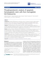
Figure 1-2: Example of a bright field image from long-term microscopy [53]
The cells are the black objects with the white halo in the images. The other small
particles are dirt.
When looking at the tracked genealogies, we observe that most siblings will differentiate
to the same type, either all MEP or all GMP. As shown in Figure 1-3, the left sub tree
has only MEPs and the right ones only GMPs. This suggests that the decision whether
the cell becomes GMP or MEP seems to be several generations ahead of when the

www.pdfgrip.com


6

1 Introduction

biological markers become active. This raises the question whether there is a way to
distinguish the cells before the onset of the currently used markers.

Figure 1-3: Labeled tracking tree of HSC differentiation to MEP or GMP [54]
Each line is branch in the tree is one linage, consisting of several cell cycles. When

the cell divides, the branch is split. Green are cell cycles with an active MEP marker,
while blue are cell cycles with an active marker for GMPs.
Two potential sources of information that have not been used for labeling so far are
the bright field images and the expression levels of other biological markers. Usually,
the bright field images are only taken for tracking purposes. However, in preliminary
studies [55] it was shown that morphological features of the cells could potentially be
used to distinguish MEPs from GMPs. Our goal is to further investigate these ideas
using innovative approaches of deep learning.

www.pdfgrip.com


1 Introduction

7

1.4 Problem Statement
The goal of this thesis is to use deep learning methods to distinguish between MEP
and GMP cells. As training data, we use sequences of bright field images for each cell
over one cycle. The cells are manually labeled, if the fluorescent level of the marker
passes a certain threshold. This problem is called supervised binary time series
classification.
We want to address this problem using deep recurrent neural networks. Despite the
advances of these models in the last years, taking raw images as input is still too
complex when dealing with time series data. Therefore, we use features describing the
shape and texture of segmented cell images. Nevertheless, these models still have to
achieve a high level of abstraction as they are presented with temporal input and have
to find patterns and similarities in time.
We want to apply our classifier to other time-lapse movies and predict the label
unknown cells. As the tracking tree suggests that the lineage choice of the cells is earlier

than the biological markers become active, we hypothesize our approach might be able
to distinguish the cells at earlier stages.

1.5 Structure of the thesis
In the first three of chapters, we give a general introduction into the techniques we are
using. First, we present basic Artificial Neural Networks and Feedfoward models that
can handle one-dimensional input. Afterwards we cover the structure as well as
problems of Recurrent Neural Networks and possible solutions on how to address these
issues. The most important part of a neural network is the training process where we
focus on the two classic optimization techniques that are still the most commonly used
approaches and different regularization techniques that prevent overfitting of the
networks when learning. Finally, we show and discuss the results of our studies and
conclude with ideas on how to continue this work.

www.pdfgrip.com


2 Introduction to deep neural networks
2.1 Feedfoward Neural Networks
Artificial Neural Networks (ANNs) are mathematical models for machine learning, that
were inspired by the structure of the central nervous system in animals or humans
[56,57]. The human brain is still the most powerful information processing unit for
complex tasks like perception, recognition and abstraction. By mimicking the biological
structure of neurons and synapses, the hope is to gain a similar capability for
understanding information and apply it to solve simple tasks.
The basic structure of an ANN is a network that consists of nodes and weighted
directed connections between these nodes. Biologically speaking, the nodes, also called
units, represent neurons and the weighted connections represent the strength of the
synapses between the neurons. To process information, a subset of the nodes is
activated, the so-called input neurons, which in turn activate other neurons by

transferring their signal. The signals are fed through the network until an output unit
is reached, which is the result of our information processing and hopefully the desired
solution.
The goal of the learning process of an ANN is to use a training set of labeled examples
and minimize a task-dependent objective function in order to achieve a good
performance on the test set, which are the examples that the model has not seen before.
In most cases, the performance can be measured by an error function that compares
the predicted with the actual labels of the data. For parametric models such as neural
networks, the error can usually be minimized by iteratively adjusting the free
parameters. The ability of an algorithm to transfer performance from the training set
to the test set is called generalization and is a key part for learning models.
Although it is now known that the models are far from the complexity of a real brain,
the methods have enjoyed continued popularity for pattern recognition and regression
tasks. Especially in recent years, with the advent of deep learning [58], a field in neural
networks where new ideas are employed to achieve a very deep structure with many
units, these models have become very powerful.

2.1.1 Perceptron
The perceptron [57] is the basic building block of an ANN and generally seen as the
first generation of neural networks. It is an algorithm for supervised binary
© Springer Fachmedien Wiesbaden 2016
M. Kroiss, Predicting the Lineage Choice of Hematopoietic Stem Cells,
BestMasters, DOI 10.1007/978-3-658-12879-1_2

www.pdfgrip.com


10

2 Introduction to deep neural networks

classification, which is able to learn the relation of data

and target

of a given set

of trainings examples. The classifier works by predicting a binary output from the data
and comparing this prediction with the correct class label. The free parameters of the
model are then iteratively adjusted in order to close the gap between predicted target
and actual target in the training set.

Input Signals

x1
x2
x3

W1

Bias parameter
Activation
Function

b

W2

v

∑

W3

φ(·)

Output
y

Summing
Junction

x4

W4
Weight parameters

Figure 2-1: Structure of a Perceptron [54]
The features of an observation
Each signal

act as input signals to the perceptron (see Figure 2-1).

is weighted by a free parameter

, which represents the influence of the

input signal on the output. The weighted signals are summed up and a bias

is added,

which can act like an offset to the linear combination. Afterwards, the combined value
is transformed by an non-linear activation function
value between 0 and 1, the sigmoid function

. To produce a binary output

(see Figure 2-2) (also called logistic

function) is used as an activation function.

Figure 2-2: Sigmoid activation function [59]

www.pdfgrip.com