Tài liệu Báo cáo khoa học: "Unsupervised Relation Disambiguation Using Spectral Clustering" ppt

Proceedings of the COLING/ACL 2006 Main Conference Poster Sessions, pages 89–96,
Sydney, July 2006.
c
2006 Association for Computational Linguistics
Unsupervised Relation Disambiguation Using Spectral Clustering
Jinxiu Chen
1
Donghong Ji
1
Chew Lim Tan
2
Zhengyu Niu
1
1
Institute for Infocomm Research
2
Department of Computer Science
21 Heng Mui Keng Terrace National University of Singapore
119613 Singapore 117543 Singapore
{jinxiu,dhji,zniu}@i2r.a-star.edu.sg
Abstract
This paper presents an unsupervised learn-
ing approach to disambiguate various rela-
tions between name entities by use of vari-
ous lexical and syntactic features from the
contexts. It works by calculating eigen-
vectors of an adjacency graph’s Laplacian
to recover a submanifold of data from a
high dimensionality space and then per-
forming cluster number estimation on the
eigenvectors. Experiment results on ACE

corpora show that this spectral cluster-
ing based approach outperforms the other
clustering methods.
1 Introduction
In this paper, we address the task of relation extrac-
tion, which is to find relationships between name en-
tities in a given context. Many methods have been
proposed to deal with this task, including supervised
learning algorithms (Miller et al., 2000; Zelenko et
al., 2002; Culotta and Soresen, 2004; Kambhatla,
2004; Zhou et al., 2005), semi-supervised learn-
ing algorithms (Brin, 1998; Agichtein and Gravano,
2000; Zhang, 2004), and unsupervised learning al-
gorithm (Hasegawa et al., 2004).
Among these methods, supervised learning is usu-
ally more preferred when a large amount of la-
beled training data is available. However, it is
time-consuming and labor-intensive to manually tag
a large amount of training data. Semi-supervised
learning methods have been put forward to mini-
mize the corpus annotation requirement. Most of
semi-supervised methods employ the bootstrapping
framework, which only need to pre-define some ini-
tial seeds for any particular relation, and then boot-
strap from the seeds to acquire the relation. How-
ever, it is often quite difficult to enumerate all class
labels in the initial seeds and decide an “optimal”
number of them.
Compared with supervised and semi-supervised
methods, Hasegawa et al. (2004)’s unsupervised ap-

proach for relation extraction can overcome the dif-
ficulties on requirement of a large amount of labeled
data and enumeration of all class labels. Hasegawa
et al. (2004)’s method is to use a hierarchical cluster-
ing method to cluster pairs of named entities accord-
ing to the similarity of context words intervening be-
tween the named entities. However, the drawback of
hierarchical clustering is that it required providing
cluster number by users. Furthermore, clustering is
performed in original high dimensional space, which
may induce non-convex clusters hard to identified.
This paper presents a novel application of spec-
tral clustering technique to unsupervised relation ex-
traction problem. It works by calculating eigenvec-
tors of an adjacency graph’s Laplacian to recover a
submanifold of data from a high dimensional space,
and then performing cluster number estimation on
a transformed space defined by the first few eigen-
vectors. This method may help us find non-convex
clusters. It also does not need to pre-define the num-
ber of the context clusters or pre-specify the simi-
larity threshold for the clusters as Hasegawa et al.
(2004)’s method.
The rest of this paper is organized as follows. Sec-
tion 2 formulates unsupervised relation extraction
and presents how to apply the spectral clustering
89
technique to resolve the task. Then section 3 reports
experiments and results. Finally we will give a con-
clusion about our work in section 4.

2 Unsupervised Relation Extraction
Problem
Assume that two occurrences of entity pairs with
similar contexts, are tend to hold the same relation
type. Thus unsupervised relation extraction prob-
lem can be formulated as partitioning collections of
entity pairs into clusters according to the similarity
of contexts, with each cluster containing only entity
pairs labeled by the same relation type. And then, in
each cluster, the most representative words are iden-
tified from the contexts of entity pairs to induce the
label of relation type. Here, we only focus on the
clustering subtask and do not address the relation
type labeling subtask.
In the next subsections we will describe our pro-
posed method for unsupervised relation extraction,
which includes: 1) Collect the context vectors in
which the entity mention pairs co-occur; 2) Cluster
these Context vectors.
2.1 Context Vector and Feature Design
Let X = {x
i
}
n
i=1
be the set of context vectors of oc-
currences of all entity mention pairs, where x
i
repre-
sents the context vector of the i -th occurrence, and n

is the total number of occurrences of all entity men-
tion pairs.
Each occurrence of entity mention pairs can be
denoted as follows:
R → (C
pre
, e
1
, C
mid
, e
2
, C
post
) (1)
where e
1
and e
2
represents the entity mentions, and
C
pre
,C
mid
,and C
post
are the contexts before, be-
tween and after the entity mention pairs respectively.
We extracted features from e
1

, e
2
, C
pre
, C
mid
,
C
post
to construct context vectors, which are com-
puted from the parse trees derived from Charniak
Parser (Charniak, 1999) and the Chunklink script
1
written by Sabine Buchholz from Tilburg University.
Words: Words in the two entities and three context
windows.
1
Software available at sabine/chunklink/
Entity Type: the entity type of both entities, which
can be PERSON, ORGANIZATION, FACIL-
ITY, LOCATION and GPE.
POS features: Part-Of-Speech tags corresponding
to all words in the two entities and three con-
text windows.
Chunking features: This category of features are
extracted from the chunklink representation,
which includes:
• Chunk tag information of the two enti-
ties and three context windows. The “0”
tag means that the word is outside of any

chunk. The “I-XP” tag means that this
word is inside an XP chunk. The “B-XP”
by default means that the word is at the
beginning of an XP chunk.
• Grammatical function of the two entities
and three context windows. The last word
in each chunk is its head, and the function
of the head is the function of the whole
chunk. “NP-SBJ” means a NP chunk as
the subject of the sentence. The other
words in a chunk that are not the head have
“NOFUNC” as their function.
• IOB-chains of the heads of the two enti-
ties. So-called IOB-chain, noting the syn-
tactic categories of all the constituents on
the path from the root node to this leaf
node of tree.
We combine the above lexical and syntactic fea-
tures with their position information in the context
to form the context vector. Before that, we filter out
low frequency features which appeared only once in
the entire set.
2.2 Context Clustering
Once the context vectors of entity pairs are prepared,
we come to the second stage of our method: cluster
these context vectors automatically.
In recent years, spectral clustering technique has
received more and more attention as a powerful ap-
proach to a range of clustering problems. Among
the efforts on spectral clustering techniques (Weiss,

1999; Kannan et al., 2000; Shi et al., 2000; Ng et al.,
2001; Zha et al., 2001), we adopt a modified version
90
Table 1: Context Clustering with Spectral-based Clustering
technique.
Input: A set of context vectors X = {x
1
, x
2
, , x
n
},
X ∈ 
n×d
;
Output: Clustered data and number of clusters;
1. Construct an affinity matrix by A
ij
= exp(−
s
2
ij
σ
2
) if i =
j, 0 if i = j. Here, s
ij
is the similarity between x
i
and

x
j
calculated by Cosine similarity measure. and the free
distance parameter σ
2
is used to scale the weights;
2. Normalize the affinity matrix A to create the matrix L =
D
−1/2
AD
−1/2
, where D is a diagonal matrix whose (i,i)
element is the sum of A’s ith row;
3. Set q = 2;
4. Compute q eigenvectors of L with greatest eigenvalues.
Arrange them in a matrix Y .
5. Perform elongated K-means with q + 1 centers on Y ,
initializing the (q + 1)-th mean in the origin;
6. If the q + 1-th cluster contains any data points, then there
must be at least an extra cluster; set q = q + 1 and go
back to step 4. Otherwise, algorithm stops and outputs
clustered data and number of clusters.
(Sanguinetti et al., 2005) of the algorithm by Ng et
al. (2001) because it can provide us model order se-
lection capability.
Since we do not know how many relation types
in advance and do not have any labeled relation
training examples at hand, the problem of model
order selection arises, i.e. estimating the “opti-
mal” number of clusters. Formally, let k be the

model order, we need to find k in Equation: k =
argmax
k
{criterion(k)}. Here, the criterion is de-
fined on the result of spectral clustering.
Table 1 shows the details of the whole algorithm
for context clustering, which contains two main
stages: 1) Transformation of Clustering Space (Step
1-4); 2) Clustering in the transformed space using
Elongated K-means algorithm (Step 5-6).
2.3 Transformation of Clustering Space
We represent each context vector of entity pair as a
node in an undirected graph. Each edge (i,j) in the
graph is assigned a weight that reflects the similarity
between two context vectors i and j. Hence, the re-
lation extraction task for entity pairs can be defined
as a partition of the graph so that entity pairs that
are more similar to each other, e.g. labeled by the
same relation type, belong to the same cluster. As a
relaxation of such NP-hard discrete graph partition-
ing problem, spectral clustering technique computes
eigenvalues and eigenvectors of a Laplacian matrix
related to the given graph, and construct data clus-
ters based on such spectral information.
Thus the starting point of context clustering is to
construct an affinity matrix A from the data, which
is an n × n matrix encoding the distances between
the various points. The affinity matrix is then nor-
malized to form a matrix L by conjugating with the
the diagonal matrix D

−1/2
which has as entries the
square roots of the sum of the rows of A. This is to
take into account the different spread of the various
clusters (points belonging to more rarified clusters
will have lower sums of the corresponding row of
A). It is straightforward to prove that L is positive
definite and has eigenvalues smaller or equal to 1,
with equality holding in at least one case.
Let K be the true number of clusters present in
the dataset. If K is known beforehand, the first K
eigenvectors of L will be computed and arranged as
columns in a matrix Y . Each row of Y corresponds
to a context vector of entity pair, and the above pro-
cess can be considered as transforming the original
context vectors in a d-dimensional space to new con-
text vectors in the K-dimensional space. Therefore,
the rows of Y will cluster upon mutually orthogonal
points on the K dimensional sphere,rather than on
the coordinate axes.
2.4 The Elongated K-means algorithm
As the step 5 of Table 1 shows, the result of elon-
gated K-means algorithm is used to detect whether
the number of clusters selected q is less than the true
number K, and allows one to iteratively obtain the
number of clusters.
Consider the case when the number of clusters q
is less than the true cluster number K present in the
dataset. In such situation, taking the first q < K
eigenvectors, we will be selecting a q-dimensional

subspace in the clustering space. As the rows of the
K eigenvectors clustered along mutually orthogo-
nal vectors, their projections in a lower dimensional
space will cluster along radial directions. Therefore,
the general picture will be of q clusters elongated in
the radial direction, with possibly some clusters very
near the origin (when the subspace is orthogonal to
some of the discarded eigenvectors).
Hence, the K-means algorithm is modified as
the elongated K-means algorithm to downweight
distances along radial directions and penalize dis-
91
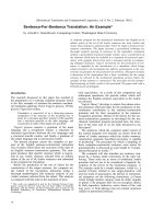
-4 -3 -2 -1 0 1 2 3 4
-4
-3
-2
-1
0
1
2
3
4
(a)
-4 -3 -2 -1 0 1 2 3 4
-4
-3
-2
-1
0
1

2
3
4
(b)
0 0.01 0.02 0.03 0.04 0.05 0.06 0.07 0.08
-0.08
-0.06
-0.04
-0.02
0
0.02
0.04
0.06
0.08
0.1
(c)
-4 -3 -2 -1 0 1 2 3 4
-4
-3
-2
-1
0
1
2
3
4
(d)
Figure 1: An Example:(a) The Three Circle Dataset.
(b) The clustering result using K-means; (c) Three
elongated clusters in the 2D clustering space using

Spectral clustering: two dominant eigenvectors; (d)
The clustering result using Spectral-based clustering
(σ
2
=0.05). (,◦ and + denote examples in different
clusters)
tances along transversal directions. The elongated
K-means algorithm computes the distance of point
x from the center c
i
as follows:
• If the center is not very near the origin, c
T
i
c
i
>  ( is a
parameter to be fixed by the user), the distances are cal-
culated as: edist(x, c
i
) = (x − c
i
)
T
M(x − c
i
), where
M =
1
λ

(I
q
−
c
i
c
T
i
c
T
i
c
i
) + λ
c
i
c
T
i
c
T
i
c
i
, λ is the sharpness param-
eter that controls the elongation (the smaller, the more
elongated the clusters)
2
.
• If the center is very near the origin,c

T
i
c
i
< , the dis-
tances are measured using the Euclidean distance.
In each iteration of procedure in Table 1, elon-
gated K-means is initialized with q centers corre-
sponding to data points in different clusters and one
center in the origin. The algorithm then will drag the
center in the origin towards one of the clusters not
accounted for. Compute another eigenvector (thus
increasing the dimension of the clustering space to
q + 1) and repeat the procedure. Eventually, when
one reach as many eigenvectors as the number of
clusters present in the data, no points will be as-
signed to the center at the origin, leaving the cluster
empty. This is the signal to terminate the algorithm.
2.5 An example
Figure 1 visualized the clustering result of three cir-
cle dataset using K-means and Spectral-based clus-
tering. From Figure 1(b), we can see that K-means
can not separate the non-convex clusters in three cir-
cle dataset successfully since it is prone to local min-
imal. For spectral-based clustering, as the algorithm
described, initially, we took the two eigenvectors of
L with largest eigenvalues, which gave us a two-
dimensional clustering space. Then to ensure that
the two centers are initialized in different clusters,
one center is set as the point that is the farthest from

the origin, while the other is set as the point that
simultaneously farthest the first center and the ori-
gin. Figure 1(c) shows the three elongated clusters in
the 2D clustering space and the corresponding clus-
tering result of dataset is visualized in Figure 1(d),
which exploits manifold structure (cluster structure)
in data.
2
In this paper, the sharpness parameter λ is set to 0.2
92
Table 2: Frequency of Major Relation SubTypes in the ACE
training and devtest corpus.
Type SubType Training Devtest
ROLE General-Staff 550 149
Management 677 122
Citizen-Of 127 24
Founder 11 5
Owner 146 15
Affiliate-Partner 111 15
Member 460 145
Client 67 13
Other 15 7
PART Part-Of 490 103
Subsidiary 85 19
Other 2 1
AT Located 975 192
Based-In 187 64
Residence 154 54
SOC Other-Professional 195 25
Other-Personal 60 10

Parent 68 24
Spouse 21 4
Associate 49 7
Other-Relative 23 10
Sibling 7 4
GrandParent 6 1
NEAR Relative-Location 88 32
3 Experiments and Results
3.1 Data Setting
Our proposed unsupervised relation extraction is
evaluated on ACE 2003 corpus, which contains 519
files from sources including broadcast, newswire,
and newspaper. We only deal with intra-sentence
explicit relations and assumed that all entities have
been detected beforehand in the EDT sub-task of
ACE. To verify our proposed method, we only col-
lect those pairs of entity mentions which have been
tagged relation types in the given corpus. Then the
relation type tags were removed to test the unsuper-
vised relation disambiguation. During the evalua-
tion procedure, the relation type tags were used as
ground truth classes. A break-down of the data by
24 relation subtypes is given in Table 2.
3.2 Evaluation method for clustering result
When assessing the agreement between clustering
result and manually annotated relation types (ground
truth classes), we would encounter the problem that
there was no relation type tags for each cluster in our
clustering results.
To resolve the problem, we construct a contin-

gency table T , where each entry t
i,j
gives the num-
ber of the instances that belong to both the i-th es-
timated cluster and j-th ground truth class. More-
over, to ensure that any two clusters do not share
the same labels of relation types, we adopt a per-
mutation procedure to find an one-to-one mapping
function Ω from the ground truth classes (relation
types) T C to the estimated clustering result EC.
There are at most |T C| clusters which are assigned
relation type tags. And if the number of the esti-
mated clusters is less than the number of the ground
truth clusters, empty clusters should be added so that
|EC| = |T C| and the one-to-one mapping can be
performed, which can be formulated as the function:
ˆ
Ω = arg max
Ω

|T C|
j=1
t
Ω(j),j
, where Ω(j) is the in-
dex of the estimated cluster associated with the j-th
class.
Given the result of one-to-one mapping, we adopt
Precision, Recall and F-measure to evaluate the
clustering result.

3.3 Experimental Design
We perform our unsupervised relation extraction on
the devtest set of ACE corpus and evaluate the al-
gorithm on relation subtype level. Firstly, we ob-
serve the influence of various variables, including
Distance Parameter σ
2
, Different Features, Context
Window Size. Secondly, to verify the effectiveness
of our method, we further compare it with other two
unsupervised methods.
3.3.1 Choice of Distance Parameter σ
2
We simply search over σ
2
and pick the value
that finds the best aligned set of clusters on the
transformed space. Here, the scattering criterion
trace(P
−1
W
P
B
) is used to compare the cluster qual-
ity for different value of σ
2 3
, which measures the ra-
tio of between-cluster to within-cluster scatter. The
higher the trace(P
−1

W
P
B
), the higher the cluster
quality.
In Table 3 and Table 4, with different settings of
feature set and context window size, we find out the
3
tr ace ( P
−1
W
P
B
) is trace of a matrix which is the sum of
its diagonal elements. P
W
is the within-cluster scatter matrix
as: P
W
=

c
j=1

X
i
∈χ
j
(X
i

− m
j
)(X
i
− m
j
)
t
and P
B
is the between-cluster scatter matrix as: P
B
=

c
j=1
(m
j
−
m)(m
j
− m)
t
, where m is the total mean vector and m
j
is
the mean vector for j
th
cluster and (X
j

− m
j
)
t
is the matrix
transpose of the column vector (X
j
− m
j
).
93
Table 3: Contribution of Different Features
Features σ
2
cluster number trace value Precison Recall F-measure
Words 0.021 15 2.369 41.6% 30.2% 34.9%
+Entity Type 0.016 18 3.198 40.3% 42.5% 41.5%
+POS 0.017 18 3.206 37.8% 46.9% 41.8%
+Chunking Infomation 0.015 19 3.900 43.5% 49.4% 46.3%
Table 4: Different Context Window Size Setting
Context Window Size σ
2
cluster number trace value Precision Recall F-measure
0 0.016 18 3.576 37.6% 48.1% 42.2%
2 0.015 19 3.900 43.5% 49.4% 46.3%
5 0.020 21 2.225 29.3% 34.7% 31.7%
corresponding value of σ
2
and cluster number which
maximize the trace value in searching for a range of

value σ
2
.
3.3.2 Contribution of Different Features
As the previous section presented, we incorporate
various lexical and syntactic features to extract rela-
tion. To measure the contribution of different fea-
tures, we report the performance by gradually in-
creasing the feature set, as Table 3 shows.
Table 3 shows that all of the four categories of fea-
tures contribute to the improvement of performance
more or less. Firstly,the addition of entity type fea-
ture is very useful, which improves F-measure by
6.6%. Secondly, adding POS features can increase
F-measure score but do not improve very much.
Thirdly, chunking features also show their great use-
fulness with increasing Precision/Recall/F-measure
by 5.7%/2.5%/4.5%.
We combine all these features to do all other eval-
uations in our experiments.
3.3.3 Setting of Context Window Size
We have mentioned in Section 2 that the context
vectors of entity pairs are derived from the contexts
before, between and after the entity mention pairs.
Hence, we have to specify the three context window
size first. In this paper, we set the mid-context win-
dow as everything between the two entity mentions.
For the pre- and post- context windows, we could
have different choices. For example, if we specify
the outer context window size as 2, then it means that

the pre-context (post-context)) includes two words
before (after) the first (second) entity.
For comparison of the effect of the outer context
of entity mention pairs, we conducted three different
Table 5: Performance of our proposed method (Spectral-
based clustering) compared with other unsupervised methods:
((Hasegawa et al., 2004))’s clustering method and K-means
clustering.
Precision Recall F-measure
Hasegawa’s Method1 38.7% 29.8% 33.7%
Hasegawa’s Method2 37.9% 36.0% 36.9%
Kmeans 34.3% 40.2% 36.8%
Our Proposed Method 43.5% 49.4% 46.3%
settings of context window size (0, 2, 5) as Table 4
shows. From this table we can find that with the con-
text window size setting, 2, the algorithm achieves
the best performance of 43.5%/49.4%/46.3% in
Precision/Recall/F-measure. With the context win-
dow size setting, 5, the performance becomes worse
because extending the context too much may include
more features, but at the same time, the noise also
increases.
3.3.4 Comparison with other Unsupervised
methods
In (Hasegawa et al., 2004), they preformed un-
supervised relation extraction based on hierarchical
clustering and they only used word features between
entity mention pairs to construct context vectors. We
reported the clustering results using the same clus-
tering strategy as Hasegawa et al. (2004) proposed.

In Table 5, Hasegawa’s Method1 means the test used
the word feature as Hasegawa et al. (2004) while
Hasegawa’s Method2 means the test used the same
feature set as our method. In both tests, we specified
the cluster number as the number of ground truth
classes.
We also approached the relation extraction prob-
lem using the standard clustering technique, K-
94
means, where we adopted the same feature set de-
fined in our proposed method to cluster the con-
text vectors of entity mention pairs and pre-specified
the cluster number as the number of ground truth
classes.
Table 5 reports the performance of our proposed
method comparing with the other two unsupervised
methods. Table 5 shows our proposed spectral based
method clearly outperforms the other two unsuper-
vised methods by 12.5% and 9.5% in F-measure re-
spectively. Moreover, the incorporation of various
lexical and syntactic features into Hasegawa et al.
(2004)’s method2 makes it outperform Hasegawa et
al. (2004)’s method1 which only uses word feature.
3.4 Discussion
In this paper, we have shown that the modified spec-
tral clustering technique, with various lexical and
syntactic features derived from the context of entity
pairs, performed well on the unsupervised relation
extraction problem. Our experiments show that by
the choice of the distance parameter σ

2
, we can esti-
mate the cluster number which provides the tightest
clusters. We notice that the estimated cluster num-
ber is less than the number of ground truth classes
in most cases. The reason for this phenomenon may
be that some relation types can not be easily distin-
guished using the context information only. For ex-
ample, the relation subtypes “Located”, “Based-In”
and “Residence” are difficult to disambiguate even
for human experts to differentiate.
The results also show that various lexical and
syntactic features contain useful information for the
task. Especially, although we did not concern the
dependency tree and full parse tree information as
other supervised methods (Miller et al., 2000; Cu-
lotta and Soresen, 2004; Kambhatla, 2004; Zhou et
al., 2005), the incorporation of simple features, such
as words and chunking information, still can provide
complement information for capturing the character-
istics of entity pairs. This perhaps dues to the fact
that two entity mentions are close to each other in
most of relations defined in ACE. Another observa-
tion from the result is that extending the outer con-
text window of entity mention pairs too much may
not improve the performance since the process may
incorporate more noise information and affect the
clustering result.
As regards the clustering technique, the spectral-
based clustering performs better than direct cluster-

ing, K-means. Since the spectral-based algorithm
works in a transformed space of low dimension-
ality, data can be easily clustered so that the al-
gorithm can be implemented with better efficiency
and speed. And the performance using spectral-
based clustering can be improved due to the reason
that spectral-based clustering overcomes the draw-
back of K-means (prone to local minima) and may
find non-convex clusters consistent with human in-
tuition.
Generally, from the point of view of unsu-
pervised resolution for relation extraction, our
approach already achieves best performance of
43.5%/49.4%/46.3% in Precision/Recall/F-measure
compared with other clustering methods.
4 Conclusion and Future work
In this paper, we approach unsupervised relation ex-
traction problem by using spectral-based clustering
technique with diverse lexical and syntactic features
derived from context. The advantage of our method
is that it doesn’t need any manually labeled relation
instances, and pre-definition the number of the con-
text clusters. Experiment results on the ACE corpus
show that our method achieves better performance
than other unsupervised methods, i.e.Hasegawa et
al. (2004)’s method and Kmeans-based method.
Currently we combine various lexical and syn-
tactic features to construct context vectors for clus-
tering. In the future we will further explore other
semantic information to assist the relation extrac-

tion problem. Moreover, instead of cosine similar-
ity measure to calculate the distance between con-
text vectors, we will try other distributional similar-
ity measures to see whether the performance of re-
lation extraction can be improved. In addition, if we
can find an effective unsupervised way to filter out
unrelated entity pairs in advance, it would make our
proposed method more practical.
References
Agichtein E. and Gravano L 2000. Snowball: Ex-
tracting Relations from large Plain-Text Collections,
In Proc. of the 5
th
ACM International Conference on
Digital Libraries (ACMDL’00).
95
Brin Sergey. 1998. Extracting patterns and relations
from world wide web. In Proc. of WebDB Workshop at
6th International Conference on Extending Database
Technology (WebDB’98). pages 172-183.
Charniak E 1999. A Maximum-entropy-inspired parser.
Technical Report CS-99-12 Computer Science De-
partment, Brown University.
Culotta A. and Soresen J. 2004. Dependency tree kernels
for relation extraction, In proceedings of 42th Annual
Meeting of the Association for Computational Linguis-
tics. 21-26 July 2004. Barcelona, Spain.
Defense Advanced Research Projects Agency. 1995.
Proceedings of the Sixth Message Understanding Con-
ference (MUC-6) Morgan Kaufmann Publishers, Inc.

Hasegawa Takaaki, Sekine Satoshi and Grishman Ralph.
2004. Discovering Relations among Named Enti-
ties from Large Corpora, Proceeding of Conference
ACL2004. Barcelona, Spain.
Kambhatla N. 2004. Combining lexical, syntactic and
semantic features with Maximum Entropy Models for
extracting relations, In proceedings of 42th Annual
Meeting of the Association for Computational Linguis-
tics. 21-26 July 2004. Barcelona, Spain.
Kannan R., Vempala S., and Vetta A 2000. On cluster-
ing: Good,bad and spectral. In Proceedings of the 41st
Foundations of Computer Science. pages 367-380.
Miller S.,Fox H.,Ramshaw L. and Weischedel R. 2000.
A novel use of statistical parsing to extract information
from text. In proceedings of 6th Applied Natural Lan-
guage Processing Conference. 29 April-4 may 2000,
Seattle USA.
Ng Andrew.Y, Jordan M., and Weiss Y 2001. On spec-
tral clustering: Analysis and an algorithm. In Pro-
ceedings of Advances in Neural Information Process-
ing Systems. pages 849-856.
Sanguinetti G., Laidler J. and Lawrence N 2005. Au-
tomatic determination of the number of clusters us-
ing spectral algorithms.In: IEEE Machine Learning
for Signal Processing. 28-30 Sept 2005, Mystic, Con-
necticut, USA.
Shi J. and Malik.J. 2000. Normalized cuts and image
segmentation. IEEE Transactions on Pattern Analysis
and Machine Intelligence. 22(8):888-905.
Weiss Yair. 1999. Segmentation using eigenvectors: A

unifying view. ICCV(2). pp.975-982.
Zelenko D., Aone C. and Richardella A 2002. Ker-
nel Methods for Relation Extraction, Proceedings of
the Conference on Empirical Methods in Natural Lan-
guage Processing (EMNLP). Philadelphia.
Zha H.,Ding C.,Gu.M,He X.,and Simon H 2001. Spec-
tral Relaxation for k-means clustering. In Neural In-
formation Processing Systems (NIPS2001). pages
1057-1064, 2001.
Zhang Zhu. 2004. Weakly-supervised relation classifi-
cation for Information Extraction, In proceedings of
ACM 13th conference on Information and Knowledge
Management (CIKM’2004). 8-13 Nov 2004. Wash-
ington D.C.,USA.
Zhou GuoDong, Su Jian, Zhang Jie and Zhang min.
2005. Exploring Various Knowledge in Relation Ex-
traction, In proceedings of 43th Annual Meeting of the
Association for Computational Linguistics. USA.
96