Tài liệu ADVANCED HIGH-SCHOOL MATHEMATICS pdf
Bạn đang xem bản rút gọn của tài liệu. Xem và tải ngay bản đầy đủ của tài liệu tại đây (3 MB, 435 trang )
Advanced High-School Mathematics
David B. Surowski
Shanghai American School
Singapore American School
January 29, 2011
i
Preface/Acknowledgment
The present expanded set of notes initially grew out of an attempt to
flesh out the International Baccalaureate (IB) mathematics “Further
Mathematics” curriculum, all in preparation for my teaching this during during the AY 2007–2008 school year. Such a course is offered only
under special circumstances and is typically reserved for those rare students who have finished their second year of IB mathematics HL in
their junior year and need a “capstone” mathematics course in their
senior year. During the above school year I had two such IB mathematics students. However, feeling that a few more students would
make for a more robust learning environment, I recruited several of my
2006–2007 AP Calculus (BC) students to partake of this rare offering
resulting. The result was one of the most singular experiences I’ve had
in my nearly 40-year teaching career: the brain power represented in
this class of 11 blue-chip students surely rivaled that of any assemblage
of high-school students anywhere and at any time!
After having already finished the first draft of these notes I became
aware that there was already a book in print which gave adequate
coverage of the IB syllabus, namely the Haese and Harris text1 which
covered the four IB Mathematics HL “option topics,” together with a
chapter on the retired option topic on Euclidean geometry. This is a
very worthy text and had I initially known of its existence, I probably
wouldn’t have undertaken the writing of the present notes. However, as
time passed, and I became more aware of the many differences between
mine and the HH text’s views on high-school mathematics, I decided
that there might be some value in trying to codify my own personal
experiences into an advanced mathematics textbook accessible by and
interesting to a relatively advanced high-school student, without being
constrained by the idiosyncracies of the formal IB Further Mathematics
curriculum. This allowed me to freely draw from my experiences first as
a research mathematician and then as an AP/IB teacher to weave some
of my all-time favorite mathematical threads into the general narrative,
thereby giving me (and, I hope, the students) better emotional and
1
Peter Blythe, Peter Joseph, Paul Urban, David Martin, Robert Haese, and Michael Haese,
Mathematics for the international student; Mathematics HL (Options), Haese and
Harris Publications, 2005, Adelaide, ISBN 1 876543 33 7
ii
Preface/Acknowledgment
intellectual rapport with the contents. I can only hope that the readers
(if any) can find some something of value by the reading of my streamof-consciousness narrative.
The basic layout of my notes originally was constrained to the five
option themes of IB: geometry, discrete mathematics, abstract algebra, series and ordinary differential equations, and inferential statistics.
However, I have since added a short chapter on inequalities and constrained extrema as they amplify and extend themes typically visited
in a standard course in Algebra II. As for the IB option themes, my
organization differs substantially from that of the HH text. Theirs is
one in which the chapters are independent of each other, having very
little articulation among the chapters. This makes their text especially
suitable for the teaching of any given option topic within the context
of IB mathematics HL. Mine, on the other hand, tries to bring out
the strong interdependencies among the chapters. For example, the
HH text places the chapter on abstract algebra (Sets, Relations, and
Groups) before discrete mathematics (Number Theory and Graph Theory), whereas I feel that the correct sequence is the other way around.
Much of the motivation for abstract algebra can be found in a variety
of topics from both number theory and graph theory. As a result, the
reader will find that my Abstract Algebra chapter draws heavily from
both of these topics for important examples and motivation.
As another important example, HH places Statistics well before Series and Differential Equations. This can be done, of course (they did
it!), but there’s something missing in inferential statistics (even at the
elementary level) if there isn’t a healthy reliance on analysis. In my organization, this chapter (the longest one!) is the very last chapter and
immediately follows the chapter on Series and Differential Equations.
This made more natural, for example, an insertion of a theoretical
subsection wherein the density of two independent continuous random
variables is derived as the convolution of the individual densities. A
second, and perhaps more relevant example involves a short treatment
on the “random harmonic series,” which dovetails very well with the
already-understood discussions on convergence of infinite series. The
cute fact, of course, is that the random harmonic series converges with
probability 1.
iii
I would like to acknowledge the software used in the preparation of
these notes. First of all, the typesetting itself made use of the indusA
try standard, LTEX, written by Donald Knuth. Next, I made use of
three different graphics resources: Geometer’s Sketchpad, Autograph,
and the statistical workhorse Minitab. Not surprisingly, in the chapter
on Advanced Euclidean Geometry, the vast majority of the graphics
was generated through Geometer’s Sketchpad. I like Autograph as a
general-purpose graphics software and have made rather liberal use of
this throughout these notes, especially in the chapters on series and
differential equations and inferential statistics. Minitab was used primarily in the chapter on Inferential Statistics, and the graphical outputs
greatly enhanced the exposition. Finally, all of the graphics were converted to PDF format via ADOBE R ACROBAT R 8 PROFESSIONAL
(version 8.0.0). I owe a great debt to those involved in the production
of the above-mentioned products.
Assuming that I have already posted these notes to the internet, I
would appreciate comments, corrections, and suggestions for improvements from interested colleagues and students alike. The present version still contains many rough edges, and I’m soliciting help from the
wider community to help identify improvements.
Naturally, my greatest debt of
gratitude is to the eleven students
(shown to the right) I conscripted
for the class. They are (back row):
Eric Zhang (Harvey Mudd), JongBin Lim (University of Illinois),
Tiimothy Sun (Columbia University), David Xu (Brown University), Kevin Yeh (UC Berkeley),
Jeremy Liu (University of Virginia); (front row): Jong-Min Choi (Stanford University), T.J. Young
(Duke University), Nicole Wong (UC Berkeley), Emily Yeh (University
of Chicago), and Jong Fang (Washington University). Besides providing one of the most stimulating teaching environments I’ve enjoyed over
iv
my 40-year career, these students pointed out countless errors in this
document’s original draft. To them I owe an un-repayable debt.
My list of acknowledgements would be woefully incomplete without
special mention of my life-long friend and colleague, Professor Robert
Burckel, who over the decades has exerted tremendous influence on how
I view mathematics.
David Surowski
Emeritus Professor of Mathematics
May 25, 2008
Shanghai, China
/>First draft: April 6, 2007
Second draft: June 24, 2007
Third draft: August 2, 2007
Fourth draft: August 13, 2007
Fifth draft: December 25, 2007
Sixth draft: May 25, 2008
Seventh draft: December 27, 2009
Eighth draft: February 5, 2010
Ninth draft: April 4, 2010
Contents
1 Advanced Euclidean Geometry
1.1 Role of Euclidean Geometry in High-School Mathematics
1.2 Triangle Geometry . . . . . . . . . . . . . . . . . . . . .
1.2.1 Basic notations . . . . . . . . . . . . . . . . . . .
1.2.2 The Pythagorean theorem . . . . . . . . . . . . .
1.2.3 Similarity . . . . . . . . . . . . . . . . . . . . . .
1.2.4 “Sensed” magnitudes; The Ceva and Menelaus
theorems . . . . . . . . . . . . . . . . . . . . . . .
1.2.5 Consequences of the Ceva and Menelaus theorems
1.2.6 Brief interlude: laws of sines and cosines . . . . .
1.2.7 Algebraic results; Stewart’s theorem and Apollonius’ theorem . . . . . . . . . . . . . . . . . . . .
1.3 Circle Geometry . . . . . . . . . . . . . . . . . . . . . . .
1.3.1 Inscribed angles . . . . . . . . . . . . . . . . . . .
1.3.2 Steiner’s theorem and the power of a point . . . .
1.3.3 Cyclic quadrilaterals and Ptolemy’s theorem . . .
1.4 Internal and External Divisions; the Harmonic Ratio . .
1.5 The Nine-Point Circle . . . . . . . . . . . . . . . . . . .
1.6 Mass point geometry . . . . . . . . . . . . . . . . . . . .
26
28
28
32
35
40
43
46
2 Discrete Mathematics
2.1 Elementary Number Theory . . . . . . . . . . . . . . . .
2.1.1 The division algorithm . . . . . . . . . . . . . . .
2.1.2 The linear Diophantine equation ax + by = c . . .
2.1.3 The Chinese remainder theorem . . . . . . . . . .
2.1.4 Primes and the fundamental theorem of arithmetic
2.1.5 The Principle of Mathematical Induction . . . . .
2.1.6 Fermat’s and Euler’s theorems . . . . . . . . . . .
55
55
56
65
68
75
79
85
v
1
1
2
2
3
4
7
13
23
vi
2.2
2.1.7 Linear congruences . . . . . . . . . .
2.1.8 Alternative number bases . . . . . .
2.1.9 Linear recurrence relations . . . . . .
Elementary Graph Theory . . . . . . . . . .
2.2.1 Eulerian trails and circuits . . . . . .
2.2.2 Hamiltonian cycles and optimization
2.2.3 Networks and spanning trees . . . . .
2.2.4 Planar graphs . . . . . . . . . . . . .
3 Inequalities and Constrained Extrema
3.1 A Representative Example . . . . . . . .
3.2 Classical Unconditional Inequalities . . .
3.3 Jensen’s Inequality . . . . . . . . . . . .
3.4 The Hălder Inequality . . . . . . . . . .
o
3.5 The Discriminant of a Quadratic . . . .
3.6 The Discriminant of a Cubic . . . . . . .
3.7 The Discriminant (Optional Discussion)
3.7.1 The resultant of f (x) and g(x) . .
3.7.2 The discriminant as a resultant .
3.7.3 A special class of trinomials . . .
.
.
.
.
.
.
.
.
.
.
.
.
.
.
.
.
.
.
.
.
.
.
.
.
.
.
.
.
.
.
.
.
.
.
.
.
.
.
.
.
.
.
.
.
.
.
.
.
.
.
.
.
.
.
.
.
.
.
.
.
.
.
.
.
.
.
.
.
.
.
.
.
.
.
.
.
.
.
.
.
.
.
.
.
.
.
.
.
.
.
.
.
.
.
.
.
.
.
.
.
.
.
.
.
.
.
.
.
.
.
.
.
.
.
.
.
.
.
.
.
.
.
.
.
.
.
.
.
.
.
.
.
.
.
.
.
145
. 145
. 147
. 155
. 157
. 161
. 167
. 174
. 176
. 180
. 182
4 Abstract Algebra
4.1 Basics of Set Theory . . . . . . . . . . . . . . . . . . .
4.1.1 Elementary relationships . . . . . . . . . . . . .
4.1.2 Elementary operations on subsets of a given set
4.1.3 Elementary constructions—new sets from old .
4.1.4 Mappings between sets . . . . . . . . . . . . . .
4.1.5 Relations and equivalence relations . . . . . . .
4.2 Basics of Group Theory . . . . . . . . . . . . . . . . .
4.2.1 Motivation—graph automorphisms . . . . . . .
4.2.2 Abstract algebra—the concept of a binary operation . . . . . . . . . . . . . . . . . . . . . . . .
4.2.3 Properties of binary operations . . . . . . . . .
4.2.4 The concept of a group . . . . . . . . . . . . . .
4.2.5 Cyclic groups . . . . . . . . . . . . . . . . . . .
4.2.6 Subgroups . . . . . . . . . . . . . . . . . . . . .
89
90
93
109
110
117
124
134
185
. 185
. 187
. 190
. 195
. 197
. 200
. 206
. 206
.
.
.
.
.
210
215
217
224
228
vii
4.2.7
4.2.8
4.2.9
Lagrange’s theorem . . . . . . . . . . . . . . . . . 231
Homomorphisms and isomorphisms . . . . . . . . 235
Return to the motivation . . . . . . . . . . . . . . 240
5 Series and Differential Equations
245
5.1 Quick Survey of Limits . . . . . . . . . . . . . . . . . . . 245
5.1.1 Basic definitions . . . . . . . . . . . . . . . . . . . 245
5.1.2 Improper integrals . . . . . . . . . . . . . . . . . 254
5.1.3 Indeterminate forms and l’Hˆpital’s rule . . . . . 257
o
5.2 Numerical Series . . . . . . . . . . . . . . . . . . . . . . 264
5.2.1 Convergence/divergence of non-negative term series265
5.2.2 Tests for convergence of non-negative term series 269
5.2.3 Conditional and absolute convergence; alternating series . . . . . . . . . . . . . . . . . . . . . . . 277
5.2.4 The Dirichlet test for convergence (optional discussion) . . . . . . . . . . . . . . . . . . . . . . . 280
5.3 The Concept of a Power Series . . . . . . . . . . . . . . . 282
5.3.1 Radius and interval of convergence . . . . . . . . 284
5.4 Polynomial Approximations; Maclaurin and Taylor Expansions . . . . . . . . . . . . . . . . . . . . . . . . . . . 288
5.4.1 Computations and tricks . . . . . . . . . . . . . . 292
5.4.2 Error analysis and Taylor’s theorem . . . . . . . . 298
5.5 Differential Equations . . . . . . . . . . . . . . . . . . . . 304
5.5.1 Slope fields . . . . . . . . . . . . . . . . . . . . . 305
5.5.2 Separable and homogeneous first-order ODE . . . 308
5.5.3 Linear first-order ODE; integrating factors . . . . 312
5.5.4 Euler’s method . . . . . . . . . . . . . . . . . . . 314
6 Inferential Statistics
317
6.1 Discrete Random Variables . . . . . . . . . . . . . . . . . 318
6.1.1 Mean, variance, and their properties . . . . . . . 318
6.1.2 Weak law of large numbers (optional discussion) . 322
6.1.3 The random harmonic series (optional discussion) 326
6.1.4 The geometric distribution . . . . . . . . . . . . . 327
6.1.5 The binomial distribution . . . . . . . . . . . . . 329
6.1.6 Generalizations of the geometric distribution . . . 330
viii
6.2
6.3
6.4
6.5
6.6
Index
6.1.7 The hypergeometric distribution . . . . . . . . . . 334
6.1.8 The Poisson distribution . . . . . . . . . . . . . . 337
Continuous Random Variables . . . . . . . . . . . . . . . 348
6.2.1 The normal distribution . . . . . . . . . . . . . . 350
6.2.2 Densities and simulations . . . . . . . . . . . . . 351
6.2.3 The exponential distribution . . . . . . . . . . . . 358
Parameters and Statistics . . . . . . . . . . . . . . . . . 365
6.3.1 Some theory . . . . . . . . . . . . . . . . . . . . . 366
6.3.2 Statistics: sample mean and variance . . . . . . . 373
6.3.3 The distribution of X and the Central Limit Theorem . . . . . . . . . . . . . . . . . . . . . . . . . 377
Confidence Intervals for the Mean of a Population . . . . 380
6.4.1 Confidence intervals for the mean; known population variance . . . . . . . . . . . . . . . . . . . 381
6.4.2 Confidence intervals for the mean; unknown variance . . . . . . . . . . . . . . . . . . . . . . . . . 385
6.4.3 Confidence interval for a population proportion . 389
6.4.4 Sample size and margin of error . . . . . . . . . . 392
Hypothesis Testing of Means and Proportions . . . . . . 394
6.5.1 Hypothesis testing of the mean; known variance . 399
6.5.2 Hypothesis testing of the mean; unknown variance 401
6.5.3 Hypothesis testing of a proportion . . . . . . . . . 401
6.5.4 Matched pairs . . . . . . . . . . . . . . . . . . . . 402
χ2 and Goodness of Fit . . . . . . . . . . . . . . . . . . . 405
6.6.1 χ2 tests of independence; two-way tables . . . . . 411
418
Chapter 1
Advanced Euclidean Geometry
1.1
Role of Euclidean Geometry in High-School
Mathematics
If only because in one’s “further” studies of mathematics, the results
(i.e., theorems) of Euclidean geometry appear only infrequently, this
subject has come under frequent scrutiny, especially over the past 50
years, and at various stages its very inclusion in a high-school mathematics curriculum has even been challenged. However, as long as we
continue to regard as important the development of logical, deductive
reasoning in high-school students, then Euclidean geometry provides as
effective a vehicle as any in bringing forth this worthy objective.
The lofty position ascribed to deductive reasoning goes back to at
least the Greeks, with Aristotle having laid down the basic foundations
of such reasoning back in the 4th century B.C. At about this time Greek
geometry started to flourish, and reached its zenith with the 13 books
of Euclid. From this point forward, geometry (and arithmetic) was an
obligatory component of one’s education and served as a paradigm for
deductive reasoning.
A well-known (but not well enough known!) anecdote describes former U.S. president Abraham Lincoln who, as a member of Congress,
had nearly mastered the first six books of Euclid. By his own admission this was not a statement of any particular passion for geometry,
but that such mastery gave him a decided edge over his counterparts
is dialects and logical discourse.
Lincoln was not the only U.S. president to have given serious thought
1
2
CHAPTER 1 Advanced Euclidean Geometry
to Euclidean geometry. President James Garfield published a novel
proof in 1876 of the Pythagorean theorem (see Exercise 3 on page 4).
As for the subject itself, it is my personal feeling that the logical
arguments which connect the various theorems of geometry are every
bit as fascinating as the theorems themselves!
So let’s get on with it ... !
1.2
1.2.1
Triangle Geometry
Basic notations
We shall gather together a few notational conventions and be reminded
of a few simple results. Some of the notation is as follows:
A, B, C
labels of points
[AB]
The line segment joining A and B
AB
The length of the segment [AB]
(AB)
The line containing A and B
A
The angle at A
C AB
The angle between [CA] and [AB]
△ABC
The triangle with vertices A, B, and C
△ABC ∼ △A′ B ′ C ′ The triangles △ABC and △A′ B ′ C ′ are congruent
=
△ABC ∼ △A′ B ′ C ′ The triangles △ABC and △A′ B ′ C ′ are similar
SECTION 1.2 Triangle Geometry
1.2.2
3
The Pythagorean theorem
One of the most fundamental results is the well-known
Pythagorean Theorem. This
states that a2 + b2 = c2 in a right
triangle with sides a and b and
hypotenuse c. The figure to the
right indicates one of the many
known proofs of this fundamental
result. Indeed, the area of the
“big” square is (a + b)2 and can be
decomposed into the area of the
smaller square plus the areas of the
four congruent triangles. That is,
(a + b)2 = c2 + 2ab,
which immediately reduces to a2 + b2 = c2 .
Next, we recall the equally wellknown result that the sum of the
interior angles of a triangle is 180◦ .
The proof is easily inferred from the
diagram to the right.
Exercises
1. Prove Euclid’s Theorem for
Proportional Segments, i.e.,
given the right triangle △ABC as
indicated, then
h2 = pq, a2 = pc, b2 = qc.
2. Prove that the sum of the interior angles of a quadrilateral ABCD
is 360◦ .
4
CHAPTER 1 Advanced Euclidean Geometry
3. In the diagram to the right, △ABC
is a right triangle, segments [AB]
and [AF ] are perpendicular and
equal in length, and [EF ] is perpendicular to [CE].
Set a =
BC, b = AB, c = AB, and deduce President Garfield’s proof1 of
the Pythagorean theorem by computing the area of the trapezoid
BCEF .
1.2.3
Similarity
In what follows, we’ll see that many—if not most—of our results shall
rely on the proportionality of sides in similar triangles. A convenient
statement is as follows.
B
Similarity. Given the similar triangles △ABC ∼ △A′ BC ′ , we have
that
′
′
′
A'
C'
′
BC
AC
AB
=
=
.
AB
BC
AC
A
C
Conversely, if
A′ B
BC ′
A′ C ′
=
=
,
AB
BC
AC
then triangles △ABC ∼ △A′ BC ′ are similar.
1
James Abram Garfield (1831–1881) published this proof in 1876 in the Journal of Education
(Volume 3 Issue 161) while a member of the House of Representatives. He was assasinated in 1881
by Charles Julius Guiteau. As an aside, notice that Garfield’s diagram also provides a simple proof
of the fact that perpendicular lines in the planes have slopes which are negative reciprocals.
SECTION 1.2 Triangle Geometry
5
Proof. Note first that △AA′ C ′
and △CA′ C ′ clearly have the same
areas, which implies that △ABC ′
and △CA′ B have the same area
(being the previous common area
plus the area of the common triangle △A′ BC ′ ). Therefore
A′ B
=
AB
=
=
=
=
1
′
2h · A B
1
2 h · AB
area △A′ BC ′
area △ABC ′
area △A′ BC ′
area △CA′ B
1 ′
′
2 h · BC
1 ′
2 h · BC
BC ′
BC
A′ C ′
A′ B
=
.
In an entirely similar fashion one can prove that
AB
AC
Conversely, assume that
B
BC ′
A′ B
=
.
AB
BC
In the figure to the right, the point
C ′′ has been located so that the segment [A′ C ′′ ] is parallel to [AC]. But
then triangles △ABC and △A′ BC ′′
are similar, and so
A
A′ B
BC ′
BC ′′
=
=
,
BC
AB
BC
A'
C"
C'
C
i.e., that BC ′′ = BC ′ . This clearly implies that C ′ = C ′′ , and so [A′ C ′ ]
is parallel to [AC]. From this it immediately follows that triangles
6
CHAPTER 1 Advanced Euclidean Geometry
△ABC and △A′ BC ′ are similar.
Exercises
1. Let △ABC and △A′ B ′ C ′ be given with ABC = A′ B ′ C ′ and
B ′C ′
A′ B ′
=
. Then △ABC ∼ △A′ B ′ C ′ .
AB
BC
A
2. In the figure to the right,
AD = rAB, AE = sAC.
Show that
D
E
Area △ADE
= rs.
Area △ABC
C
B
3. Let △ABC be a given triangle and let Y, Z be the midpoints of
[AC], [AB], respectively. Show that (XY ) is parallel with (AB).
(This simple result is sometimes called the Midpoint Theorem)
B
4. In △ABC, you are given that
Z
AY
CX
BX
1
=
=
= ,
YC
XB
ZA
x
where x is a positive real number.
Assuming that the area of △ABC
is 1, compute the area of △XY Z as
a function of x.
X
C
Y
A
5. Let ABCD be a quadrilateral and let EF GH be the quadrilateral
formed by connecting the midpoints of the sides of ABCD. Prove
that EF GH is a parallelogram.
SECTION 1.2 Triangle Geometry
7
6. In the figure to the right, ABCD is
a parallelogram, and E is a point
on the segment [AD]. The point
F is the intersection of lines (BE)
and (CD). Prove that AB × F B =
CF × BE.
7. In the figure to the right, tangents
to the circle at B and C meet at the
point A. A point P is located on
˘
the minor arc BC and the tangent
to the circle at P meets the lines
(AB) and (AC) at the points D and
E, respectively. Prove that DOE =
1
2 B OC, where O is the center of the
given circle.
1.2.4
“Sensed” magnitudes; The Ceva and Menelaus theorems
In this subsection it will be convenient to consider the magnitude AB of
the line segment [AB] as “sensed,”2 meaning that we shall regard AB
as being either positive or negative and having absolute value equal to
the usual magnitude of the line segment [AB]. The only requirement
that we place on the signed magnitudes is that if the points A, B, and
C are colinear, then
>
AB × BC =
2
<
−→
−→
−→
−→
0
if AB and BC are in the same direction
0
if AB and BC are in opposite directions.
IB uses the language “sensed” rather than the more customary “signed.”
8
CHAPTER 1 Advanced Euclidean Geometry
This implies in particular that for signed magnitudes,
AB
= −1.
BA
Before proceeding further, the reader should pay special attention
to the ubiquity of “dropping altitudes” as an auxiliary construction.
Both of the theorems of this subsection are concerned with the following
configuration: we are given the triangle △ABC and points X, Y, and Z on
the lines (BC), (AC), and (AB), respectively. Ceva’s Theorem is concerned with
the concurrency of the lines (AX), (BY ),
and (CZ). Menelaus’ Theorem is concerned with the colinearity of the points
X, Y, and Z. Therefore we may regard these theorems as being “dual”
to each other.
In each case, the relevant quantity to consider shall be the product
AZ BX CY
×
×
ZB XC Y A
Note that each of the factors above is nonnegative precisely when the
points X, Y, and Z lie on the segments [BC], [AC], and [AB], respectively.
The proof of Ceva’s theorem will be greatly facilitated by the following lemma:
SECTION 1.2 Triangle Geometry
9
Lemma.
Given the triangle
△ABC, let X be the intersection of
a line through A and meeting (BC).
Let P be any other point on (AX).
Then
area △APB BX
=
.
area △APC CX
Proof. In the diagram to the
right, altitudes BR and CS have
been constructed. From this, we see
that
area △APB
=
area △APC
1
2 AP
1
2 AP
BR
CS
BX
,
=
CX
· BR
· CS
=
where the last equality follows from the obvious similarity
△BRX ∼ △CSX.
Note that the above proof doesn’t depend on where the line (AP ) intersects (BC), nor does it depend on the position of P relative to the
line (BC), i.e., it can be on either side.
Ceva’s Theorem. Given the triangle △ABC, lines (usually called
Cevians are drawn from the vertices A, B, and C, with X, Y , and Z,
being the points of intersections with the lines (BC), (AC), and (AB),
respectively. Then (AX), (BY ), and (CZ) are concurrent if and only
if
AZ BX CY
×
×
= +1.
ZB XC Y A
10
CHAPTER 1 Advanced Euclidean Geometry
Proof. Assume that the lines in question are concurrent, meeting in
the point P . We then have, applying the above lemma three times,
that
area △APC area △APB area △BPC
·
·
area △BPC area △APC area △BPA
AZ BX CY
=
·
·
.
ZB XC Y A
1 =
.
To prove the converse we need to
prove that the lines (AX), (BY ),
and (CZ) are concurrent, given
that
AZ BX CY
·
·
= 1.
ZB XC Y Z
Let Q = (AX) ∩ (BY ), Z ′ =
(CQ) ∩ (AB). Then (AX), (BY ),
and (CZ ′ ) are concurrent and so
AZ ′ BX CY
·
·
= 1,
Z ′ B XC Y Z
which forces
AZ ′
AZ
=
.
Z ′B
ZB
This clearly implies that Z = Z ′ , proving that the original lines (AX), (BY ),
and (CZ) are concurrent.
Menelaus’ theorem is a dual version of Ceva’s theorem and concerns
not lines (i.e., Cevians) but rather points on the (extended) edges of
SECTION 1.2 Triangle Geometry
11
the triangle. When these three points are collinear, the line formed
is called a transversal. The reader can quickly convince herself that
there are two configurations related to △ABC:
As with Ceva’s theorem, the relevant quantity is the product of the
sensed ratios:
AZ BX CY
·
·
;
ZB XC Y A
in this case, however, we see that either one or three of the ratios must
be negative, corresponding to the two figures given above.
Menelaus’ Theorem. Given the triangle △ABC and given points
X, Y, and Z on the lines (BC), (AC), and (AB), respectively, then
X, Y, and Z are collinear if and only if
AZ BX CY
×
×
= −1.
ZB XC Y A
Proof. As indicated above, there are two cases to consider. The first
case is that in which two of the points X, Y, or Z are on the triangle’s
sides, and the second is that in which none of X, Y, or Z are on the
triangle’s sides. The proofs of these cases are formally identical, but
for clarity’s sake we consider them separately.
12
CHAPTER 1 Advanced Euclidean Geometry
Case 1. We assume first that
X, Y, and Z are collinear and drop
altitudes h1 , h2 , and h3 as indicated
in the figure to the right. Using obvious similar triangles, we get
AZ
h1 BX
h2 CY
h3
=+ ;
=+ ;
=− ,
ZB
h2 XC
h3 Y A
h1
in which case we clearly obtain
AZ BX CY
×
×
= −1.
ZB XC Y A
To prove the converse, we may assume that X is on [BC], Z is on
AZ
[AB], and that Y is on (AC) with ZB · BX · CY = −1. We let X ′ be the
XC Y A
intersection of (ZY ) with [BC] and infer from the above that
AZ BX ′ CY
·
·
= −1.
ZB X ′ C Y A
′
It follows that BX = BX , from which we infer easily that X = X ′ , and
XC
X ′C
so X, Y, and Z are collinear.
Case 2. Again, we drop altitudes from
A, B, and C and use obvious similar triangles, to get
AZ
h1 BX
h2 AY
h1
=− ;
=− ;
=− ;
ZB
h2 XC
h3 Y C
h3
it follows immediately that
AZ BX CY
·
·
= −1.
ZB XC Y A
The converse is proved exactly as above.
SECTION 1.2 Triangle Geometry
1.2.5
13
Consequences of the Ceva and Menelaus theorems
As one typically learns in an elementary geometry class, there are several notions of “center” of a triangle. We shall review them here and
show their relationships to Ceva’s Theorem.
Centroid. In the triangle △ABC
lines (AX), (BY ), and (CZ)
are drawn so that (AX) bisects
[BC], (BY ) bisects [CA], and
(CZ) bisects [AB] That the lines
(AX), (BY ), and (CZ) are concurrent immediately follows from
Ceva’s Theorem as one has that
AZ BX CY
·
·
= 1 × 1 × 1 = 1.
ZB XC Y Z
The point of concurrency is called the centroid of △ABC. The three
Cevians in this case are called medians.
Next, note that if we apply the Menelaus’ theorem to the triangle
△ACX and the transversal defined by the points B, Y and the centroid
P , then we have that
1=
AY CB XP
·
·
⇒
Y C BX P A
1=1·2·
XP
XP
1
⇒
= .
PA
PA
2
Therefore, we see that the distance of a triangle’s vertex to the centroid
is exactly 1/3 the length of the corresponding median.
14
CHAPTER 1 Advanced Euclidean Geometry
Orthocenter.
In the triangle △ABC lines (AX), (BY ), and
(CZ) are drawn so that (AX) ⊥
(BC), (BY ) ⊥ (CA), and (CZ) ⊥
(AB). Clearly we either have
AZ BX CY
,
,
>0
ZB XC Y A
or that exactly one of these ratios
is positive. We have
△ABY ∼ △ACZ ⇒
CZ
AZ
=
.
AY
BY
Likewise, we have
△ABX ∼ △CBZ ⇒
AX
BX
=
and △CBY ∼ △CAX
BZ
CZ
⇒
CY
BY
=
.
CX
AX
Therefore,
AZ BX CY
AZ BX CY
CZ AX BY
·
·
=
·
·
=
·
·
= 1.
ZB XC Y A
AY BZ CX
BY CZ AX
By Ceva’s theorem the lines (AX), (BY ), and (CZ) are concurrent, and
the point of concurrency is called the orthocenter of △ABC. (The
line segments [AX], [BY ], and [CZ] are the altitudes of △ABC.)
Incenter. In the triangle △ABC lines
(AX), (BY ), and (CZ) are drawn so
that (AX) bisects B AC, (BY ) bisects
ABC, and (CZ) bisects B CA As we
show below, that the lines (AX), (BY ),
and (CZ) are concurrent; the point of
concurrency is called the incenter of
△ABC. (A very interesting “extremal”
SECTION 1.2 Triangle Geometry
15
property of the incenter will be given in
Exercise 12 on page 153.) However, we shall proceed below to give
another proof of this fact, based on Ceva’s Theorem.
Proof that the angle bisectors of △ABC are concurrent. In
order to accomplish this, we shall first prove the
Angle Bisector Theorem. We
are given the triangle △ABC with
line segment [BP ] (as indicated to
the right). Then
AP
AB
=
⇔ ABP = P BC.
BC
PC
Proof (⇐). We drop altitudes
from P to (AB) and (BC); call the
points so determined Z and Y , respectively. Drop an altitude from
B to (AC) and call the resulting
point X. Clearly P Z = P Y as
△P ZB ∼ △P Y B. Next, we have
=
△ABX ∼ △AP Z ⇒
BX
BX
AB
=
=
.
AP
PZ
PY
Likewise,
△CBX ∼ △CP Y ⇒
BX
CB
=
.
CP
PY
Therefore,
AP · BX
PY
AP
AB
=
·
=
.
BC
PY
CP · BX
CP