Wolfgang walter ordinary differential equations (1998) 978 1 4612 0601 9

www.pdfgrip.com


Graduate Texts in Mathematics
Readings in Mathematics
Ebbinghaus/Hermes/Hirzebruch/Koecher/MainzerlNeukirch/Prestel/Remmert: Mlmbas
Fulton/Han"is: Representation 771eOI)': A First COllrse
Remmert: TheolY of Complex FlInctions

Undergraduate Texts in Mathematics
Readings in Mathematics
Anglin: Mathematics: A Concise HislOIJ' and Philosophy
Anglin/Lambek: The Heritage of Thales
Bressoud: Second Year Calcllills
Hairer/Wanner: Analysis by Its History
Hammerlin/Hoffmann: NlImerical Mathematics
Isaac: The Pleasllres of Probability
Samuel: Projective Geometrl'
Stillwell: NlImbers and Geometry
Toth: Glimpses of Algebra and Geomelt)'

www.pdfgrip.com


Wolfgang Walter

Ordinary Differential
Equations
Translated by Russell Thompson

,

Springer

www.pdfgrip.com


Wolfgang Walter
Mathematisches Institut I
Universităt Karlsruhe
D-76128 Karlsruhe
Germany

Russell Thompson
Utah State University
College of Science
Department of Mathematics and Statistics
Logan, UT 84322-3900

Editorial Board
S. Axler
Mathematics Department
San Francisco State
University
San Francisco, CA 94132
USA

F.W. Gehring
Mathematics Department
East Hali

University of Michigan
Ann Arbor, MI 48109
USA

K.A. Ribet
Mathematics Department
University of California
at Berkeley
Berkeley, CA 94720-3840
USA

Mathematics Subject Clas8ification (1991): 34-01
Library of Congress Cataloging-in-Publication Data
Walter, Wolfgang, 1927Ordinary differential equations / Wolfgang Walter.
p.
cm. - (Graduate texts in mathematics ; 182. Readings in
mathematics)
Includes bibliographical references and index.
ISBN 978-1-4612-6834-5
ISBN 978-1-4612-0601-9 (eBook)
DOI 10.1007/978-1-4612-0601-9
1. Differential equations. 1. Title.

II. Series: Graduate texts
in mathematics ; 182. III. Series: Graduate texts in mathematics.
Readings in mathematics.
QA372.W224 1998
515'.352--dc21
98-4754
Printed on acid-free paper.

© 1998 Springer Science+Business Media New York
Original1y published by Springer-Verlag New York, Inc. in 1998
Softcover reprint ofthe hardcover 18t edition 1998
AII rights reserved. This work may not be translated or copied in whole or in part without the
written permission of the publisher Springer Science+Business Media., LLC.
except for brief excerpts in connection with reviews or scholarly analysis. Use
in connection with any form of information storage and retrieva!, electronic adaptation, computer
software, Of by similar or dissimilar methodology now known or hereafter developed is forbidden.
The use of general descriptive names. trade namcs. trademarks. etc .. in this pub1ication, even if the
former are not especially identified, is not to be taken as a sign that such names, as understood by
the Trade Marks and Merchandise Marks Act, may accordingly be used freely by anyone.

Production managed by Alian Abrams; manufacturing supervised by Jacqui Ashri.
Photocomposed copy prepared from the translator's TeX files.
987654321
ISBN 978-1-4612-6834-5

www.pdfgrip.com


Preface
The author's book on Gewohnliche Differentialgleichungen (Ordinary Differential Equations) was published in 1972. The present book is based on a
translation of the latest, 6th, edition, which appeared in 1996, but it also treats
some important subjects that are not found there. The German book is widely
used as a textbook for a first course in ordinary differential equations. This is
a rigorous course, and it contains some material that is more difficult than that
usually found in a first course textbook; such as, for example, Peano's existence
theorem. It is addressed to students of mathematics, physics, and computer science and is usually taken in the third semester. Let me remark here that in the
German system the student learns calculus of one variable at the gymnasium 1
and begins at the university with a two-semester course on real analysis which

is usually followed by ordinary differential equations.
Prerequisites. In order to understand the main text, it suffices that the
reader have a sound knowledge of calculus and be familiar with basic notions
from linear algebra. For complex differential equations, some facts about holomorphic functions and their integrals are required. These are summarized at
the beginning of § 8 and more fully described and partly proved in part C of the
Appendix. Functional analysis is developed in the text when needed. In several
places there are sections denoted as Supplements, where more special subjects
are treated or the theory is extended. More advanced tools such as Lebesgue's
theory of integration or Schauder's fixed point theorem are occasionally used in
those sections. The supplements and also § 13 can be omitted in a first reading.
Outline of contents. The book treats significantly more topics than can
be covered in a one-semester course. It also contains material that is seldom
found in textbooks and-what is perhaps more important-it uses new proofs
for basic theorems. This aspect of the book calls for a closer look at contents and
methods with emphasis on those places where we depart from the mainstream.
The first chapter treats classical cases of first order equations that can be
solved explicitly. By means of a number of examples the student encounters the
essential features of the initial value problem such as uniqueness and nonuniqueness, maximal solutions in the case of nonuniqueness, and continuous dependence on initial values in the small, but not in the large; see l.VI-VIII. The
1 In the German school system, the gymnasium is an academic high school that prepares
students for study at the university.

v

www.pdfgrip.com


VI

Preface

phase plane and phase portraits are explained in 3.VI-VIII.
The theory proper starts with Chapter II. In this and the following chapter
the initial value problem is treated first for one equation and then for systems
of equations. The repetition caused by this separation of cases is minimal since
all proofs carryover, while the student has the benefit that the reasoning is not
burdened by technicalities about vector functions. The complex case, where
the solutions are holomorphic functions, is treated in § 8; the proofs follow the
pattern set in § 6 for the real case. The theory of differential inequalities in §
9 is one-dimensional by its very nature. An extension to n dimensions leads to
new phenomena that are treated in Supplement I of § 10.
Chapter IV is devoted to linear systems and linear differential equations of
higher order. In a Supplement to § 18 the Floquet theory for systems with
periodic coefficients is presented.
Linear systems in the complex domain is the topic of Chapter V. The main
properties of systems with isolated singularities are developed in a novel way
(see below). Equations of mathematical physics are discussed in § 25.
The main subject of Chapter VI is the Sturm-Liouville theory of boundary
value and eigenvalue problems. Nonlinear boundary value problems and corresponding existence, uniqueness, and comparison theorems are also treated. In
§ 28 the eigenvalue theory for compact self-adjoint operators in Hilbert space is
developed and applied to the Sturm-Liouville eigenvalue problem.
The last chapter deals with stability and asymptotic behavior of solutions.
The linearization theorem of Grobman-Hartman is given without proof (the
author is still looking for a rea]]y good proof). The method of Lyapunov is
developed and applied in § 30.
An appendix consisting of four parts A (topology), B (real analysis), C
(complex analysis), and D (functional analysis) contains notions and theorems
that are used in the text or can lead to a deeper understanding of the subject.
The fixed point theorems of Brouwer and Schauder are proved in B.V and D.XII.
In closing this overview, we point out that applications, mostly from mechanics and mathematical biology, are found in many places. Exercises, which
range from routine to demanding, are dispersed throughout the text, some with

an outline of the solution. Solutions of selected exercises are found at the end
of the book.
Special Features. Two general themes exercise a profound influence throughout the book: functional analysis and differential inequalities.
Functional Analysis. The contraction principle, that is, the fixed point
theorem for contractive mappings in a Banach space, is at the center. This theorem has all necessary properties to make it a fundamental principle of analysis:
It is elementary, widely applicable, and far-reaching. 2 Its flexibility in connection with our subject comes to light when appropriate weighted maximum norms
2 A remarkable theorem of Bessaga (1959) sheds light on the versatility of the contraction
principle. Consider a map T : 5 ---> 5, where 5 is an arbitrary set, and assume that T has a
unique fixed point which is also the only fixed point of T 2 , T 3 , .... Then there is a metric on
5 that makes 5 a complete metric space and T a contraction. One can even find metrics for
which the Lipschitz constant of T is arbitrarily small.

www.pdfgrip.com


Preface

vii

are used. A first example is found in the dissertation of Morgenstern (1952);
references to later authors in the literature are historically unjustified. In linear
complex systems, the weighted maximum norm in 21.11 leads to global existence
without using analytic continuation and the monodromy theorem. Moreover,
this proof gives the growth properties of solutions that are needed in the treatment of singular points. The theorems on continuous dependence on initial
values and parameters and on holomorphy with regard to complex parameters
follow directly from the contraction principle, a fact which is still little known.
Differentiability with respect to real parameters requires Ostrowski's theorem
on approximate iteration 13.IV.
In the treatment of linear systems with weakly singular points, the crucial
convergence proofs are also reduced to the contraction principle in a suitable

Banach space. 3 For holomorphic solutions, i.e., power series expansions, this
method was discovered by Harris, Sibuya, and Weinberg (1969). The logarithmic case can also be treated along these lines. This approach leads also to
theorems of Lettenmeyer and others, which are beyond the scope of this book;
cf. the original work cited above.
A theorem in Appendix D.VII, which is partly due to Holmes (1968), establishes a relation between the norm of a linear operator and its spectral radius.
As explained in Section D.IX, this result gives a better insight into the role of
weighted maximum norms.
Differential Inequalities. The author, who also wrote the first monograph
on differential inequalities (1964, 1970), has encountered many instances where
authors are unaware of basic theorems on differential inequalities that would
have made their reasoning much simpler and stronger. The distinction between
weak and strong inequalities is a matter of fundamental importance. In partial
differential equations this is common knowledge: weak maximum or comparison
principles versus strong principles of this type. Not so in ordinary differential
equations. Theorem 9.IX is a strong comparison principle that prescribes precisely the occurrence of strict inequalities, while most (all?) textbooks are content with the weak "less than or equal" statement. This principle is essential
for our treatment of the Sturm-Liouville theory via Prufer transformation. Its
usefulness in nonlinear Sturm theory can be seen from a recent paper, "Valter
(1997).
Supplement I in § 10 brings the two basic theorems on systems of differential inequalities, (i) the comparison theorem for quasimonotone systems, and (ii)
Max Muller's theorem for the general case. Both were found in the mid twenties. Q'Uasimonotonicity is a necessary and sufficient condition for extending the
classical theory (including maximal and minimal solutions) from one equation
to systems of equations. More recently, both theorems (i) and (ii) have been
applied to population dynamics, but it is not generally known that results on
3The Banach space H o of 24.1, which is indeed a Banach algebra, can be used for a short
and elegant proof of two fundamental theorems for functions of several complex variables, the
preparation theorem and the division theorem of vVeierstrass. This proof has been propagated
by Grauert and Remmert since the sixties and can be found, e.g., in their book Coher-ent
Analytic Sheaves (Grundlehren 265, Springer 1984); d. \""alter (1992) for other applications.

www.pdfgrip.com

viii

Preface

invariant rectangles are special cases of Muller's theorem. Theorem 1O.XII is
the strong version of (i); it contains M. Hirsch's theorem on strongly monotone
flows, cf. Hirsch (1985) and Walter (1997).
A Supplement to § 26 describes a new approach to minimum principles for
boundary value problems of Sturmian type that applies also to nonlinear differential operators; cf. Walter (1995). The strong minimum principle is generalized
in 26.XIX, so that it includes now the first eigenvalue case.
In Supplement II of § 26 on nonlinear boundary value problems the method
of upper and lower solutions for existence and Serrin's sweeping principle for
uniqueness are presented.
Miscellaneous Topics. Differ-ential equations in the sense oj Caratheodor-y. The initial value problem is treated in Supplement II of § 10 and a SturmLiouville theory under Caratheodory assumptions in 26,XXIV and 27.XXI. As a
rule, the earlier proofs for the classical case carryover. This applies in particular
to the strong comparison theorem 1O.XV and the strong minimum principle in
26.XXV.
Radial solutions of elliptic equations. This subject plays an active role in
recent research on nonlinear elliptic problems. The radial ~-operator is an operator of Sturm-Liouville type with a singularity at O. The corresponding initial
value problem is treated in a supplement of § 6, and the eigenvalue problem and
nonlinear boundary value problems for the unit ball in \R.n (for radial solutions)
in a Supplement to § 27.
Separatr-ices is the theme of a Supplement in § 9. Differential inequalites are
essential for proving existence and uniqueness.
Special Applications. We mention the generalized logistic equation in a supplement to § 2, general predator-prey models in 3.VII, delay-differential equations in 7.XIV-XV, invariant sets in 10.XVI and the rubber band as a model for
nonlinear oscillations in a nonsymmetric mechanical system in 11.X.
Exact Numer-ics. vVe give examples in which a combination of a numerical
procedure and a sup-superfunction technique allows a mathematically exact

computation of special values. The numerical part is based on an algorithm,
developed by Rudolf Lohner (1987, 1988), that computes exact enclosures for
the solutions of an initial value problem. In blow-up problems one obtains rather
sharp enclosures for the location of the asymptote of the solutions; cf. 9.V. A
different kind of sub- and supersolutions is used to compute a separatrix; in
general, a separatrix is an unstable solution.
Acknowledgments. It is a pleasure to thank all those who have contributed
to the making of this volume. The translator, Professor Russell Thompson,
worked with expertise and patience in the face of changes and additions during
the translation and furnished beautiful figures. He also suggested an improved
division into chapters. Irene Redheffer acted as a mediator between author and
translator with exceptional care and insight and translated the Solutions section.
Her help and advice and that of Professor Ray Redheffer were indispensable.
My sincere thanks go to all of them and also to other helping hands and minds.
K aTlsruhe, August 1997

Wolfgang Walter

www.pdfgrip.com


Table of Contents
Preface

v

Note to the Reader

xi

Introduction

1

Chapter I. First Order Equations: Some Integrable Cases
§ 1. Explicit First Order Equations . . . . . . . . . . . .
§ 2. The Linear Differential Equation. Related Equations . . .
Supplement: The Generalized Logistic Equation . . . .
§ 3. Differential Equations for Families of Curves. Exact Equations
§ 4. Implicit First Order Differential Equations. . . . . . . .

9
9
27
33
36
46

Chapter II: Theory of First Order Differential Equations
§ 5. Tools from Functional Analysis . . . . . . . . .
§ 6. An Existence and Uniqueness Theorem
Supplement: Singular Initial Value Problems
§ 7. The Peano Existence Theorem
Supplement: Methods of Functional Analysis
§ 8. Complex Differential Equations. Power Series Expansions
§ 9. Upper and Lower Solutions. Maximal and lVlinimal Integrals
Supplement: The Separatrix . . . . . . . . . . . . . . . . .

53
53

62
70
73
80
83
89
98

Chapter III: First Order Systems. Equations of Higher Order
§ 10. The Initial Value Problem for a System of First Order .
Supplement I: Differential Inequalities and Invariance
Supplement II: Differential Equations in the Sense
of Caratheodory . . . . . . . . . . .
§ 11. Initial Value Problems for Equations of Higher Order.
Supplement: Second Order Differential Inequalities
§ 12. Continuous Dependence of Solutions . . . . . . . . . .
Supplement: General Uniqueness and Dependence Theorems
§ 13. Dependence of Solutions on Initial Values and Parameters
IX

www.pdfgrip.com

105
105
111
121
125
139
141
146

148


x

Table of Contents

Chapter IV: Linear Differential Equations
§ 14. Linear Systems
.
§ 15. Homogeneous Linear Systems . . . . . .
§ 16. Inhomogeneous Systems
.
Supplement: L1-Estimation of C-Solutions
§ 17. Systems with Constant Coefficients . . . . .
§ 18. Matrix Functions. Inhomogeneous Systems
Supplement: Floquet Theory . . . . . . .
§ 19. Linear Differential Equations of Order n ..
§ 20. Linear Equations of Order n with Constant Coefficients
Supplement: Linear Differential Equations with
Periodic Coefficients . . . . . . . . . . . . . . .

159

Chapter V: Complex Linear Systems
§ 21. Homogeneous Linear Systems in the Regular Case
§ 22. Isolated Singularities . . . . . . . . . . . . . . . . .
§ 23. Weakly Singular Points. Equations of Fuchsian Type
§ 24. Series Expansion of Solutions .
§ 25. Second Order Linear Equations . . . . . . . . . . . .

213

Chapter VI: Boundary Value and Eigenvalue Problems
§ 26. Boundary Value Problems . . . . . . . . . . . . . . . .
Supplement 1: Nlaximum and Minimum Principles .
Supplement II: Nonlinear Boundary Value Problems
§ 27. The Sturm-Liouville Eigenvalue Problem
.
Supplement: Rotation-Symmetric Elliptic Problems
§ 28. Compact Self-Adjoint Operators in Hilbert Space

245

Chapter VII: Stability and Asymptotic Behavior
§ 29. Stability . . . . . . . . ..
§ 30. The Method of Lyapunov

305

159
164
170

173
175
190
195
198
204

210
213
216
222
225
236
245
260
262
268
281
286
305
. 318

Appendix
A. Topology
.
B. Real Analysis
.
C. Complex Analysis
D. Functional Analysis .

333

Solutions and Hints for Selected Exercises

357

Literature

367

Index

372

Notation

379

333
342
348
350

www.pdfgrip.com


Note to the Reader
In references to another paragraph. the number of the paragraph is given
before the number of the formula, theorem, lemma.. . .. For example, formula
(7) in § 15 is denoted as (15.7), and theorem 15.III or corollary 15.III refers to
the theorem or corollary in section III of § 15. But when citing within § 15, we
write simply formula (7), Theorem III, and Corollary III. A reference to B.V
refers to Section V in Part B of the Appendix.
When the name of an author is followed by the year of publication, as in
Perron (1926), the source is found in the bibliography at the end of the book.
lVly two books on analysis are cited as Walter 1 and Walter 2. A compilation of
general notions and a list of symbols are found at the end of the book.

The German word Ansatz is used repeatedly: a footnote in Part II of the
introduction gives an explanation.

xi

www.pdfgrip.com


Introduction
A differential equation is an equation containing independent variables, functions, and derivatives of functions. The equation
y/

+ 2;ry = 0

(1)

is a differential equation. Here x is the independent variable and y is the unknown function. A solution is a function y = ¢( x) that satisfies (1) identically
.2
in x, that is, ¢/ (x) + 2x· ¢(x) = O. It is easy to check that the function y = e- x
is a solution of (1):
d.2

2

_(e- X )+2xe- x =0
dx

for

-oo

We will see later that the collection of all solutions of (1) can be written in the
2
form y = C . e- X , where C runs through the set of real numbers.
Equation (1) is a differential equation of first order. The general differential
equation of first order has the form

(2)

F(x, y, y/) = O.

A function y = y(x) is called a solution of (2) in an interval J if y(x) is differentiable in J and
F(x, y(x), y/(x))

=0

holds for all x E J.

If a differential equation contains higher order derivatives, say up to nth
order, then the equation is called an nth order differential equation. Such an
equation can always be written in the general form
I
- 0
.
F( x,y,y,
... ,y (n)) .

(3)

Here a solution is defined to be an n-times differentiable function such that

equation (3) is satisfied identically when y(x) and its derivatives are substituted
into F. A differential equation of nth order is called explicit if it has the form
yin)

=

f(x, y, y/, ... , y(n-l));

(4)

otherwise it is called implicit. For a first order ordinary differential equation the
explicit form is

y/

=

f(x, y).

(5)
1

www.pdfgrip.com


2

Introduction

The above comments apply to ordinary differential equations, that is, to

differential equations for functions y(x) of a single independent variable x. If
several independent variables and hence also partial derivatives are present, then
the equation is called a par·tial differential eq·uation. For example,
Ux

+ Uy =

x

+y

is a partial differential equation of first order for an unknown function u(x,y).
The function U(.T, y) = xy is a particular solution to this equation. An important
example of a second order partial differential equation is the potent'ial equation
in three-space
t:,.u

==

U.TX

+ U yy + U zz = 0,

where u = u(x,y,z).
In this book we will be concerned only with ordinary differential equations.
The primary emphasis will be on differential equations in the real domain where
the independent variable x is a real variable and y(x) is a real function. However,
the fundamental facts about differential equations in the complex domain will
also be treated.
The expression -integral of a differential equat-ion is another term used for a

solut'ion, and the terms solution curve and integral curve are used to emphasize
the geometric interpretation of a solution as a curve. A family of functions
y(x; e l , ... , en), depending on x and n parameters e l , ... , en (which vary in a
point set A1 c IR n ). is called a complete -integral or a general solution of the nth
order differential equation (4) if it satisfies the following two requirements: first,
each function y(:r:; e l •... , en) is a solution to the differential equation (4) for an
arbitrary choice of the parameters (el , ... , en) E 1\1, and second, all solutions
can be obtained in this manner. The notion of a general solution does not play
a major role in the theory of differential equations. It is used here in connection
with simple examples, where it is actually possible to give all solutions explicitly
in a form depending 011 n parameters.
Differential equations playa cardinal role in the natural sciences and technology, especially in physics. for the simple reason that many physical laws take
the form of a differential equation. Differential equations also appear in other
scientific domains where mathernaticalmodels and theories are used. The three
examples that follow are intended to give a first impression of the type of problems that arise. They all deal with the motion of a body in a gravitational
field.
I. Free Fall. W'hen a body at rest is suddenly released, it falls downward
under the influence of gravity. This motion can be described mathematically
by a fUllction s = s(t) which gives the distance that the body (or more exactly,
its center of mass) has traveled up to time t. Other quantities of interest that
d
can be derived frol11 8 include the instantaneous velocity v(t) = ~d s(t) = s(t)
t
d
and the acceleration a(t) = ~v(t) = s(t). (When describing processes in which
dt

www.pdfgrip.com

Introduction

3

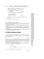
o
1
2

3
4

the independent variable represents time, it is customary to denote the independent variable by t instead of x, and derivatives by dots instead of primes.)
We learn in elementary mechanics that the acceleration of such bodies may be
assumed to be constant, in fact, equal to the acceleration g due to gravity at the
earth's surface. Thus the distance-time function s(t) satisfies the second order
differential equation

s=

(6)

g.

It is easy to find all of the solutions here. Indeed. it follows from integrating the
equation v(t) = g that v(t) = gt + C j • and likewise from 8(t) = gt + C j that
1
2

s(t) = -gt

2

+ Cjt + C2

(C 1 . C2 constant).

We have thus found the complete integral of the differential equation (6).
To go from this family of s = g to the solution that corresponds to a particular physical process requires some additional information. the so-called initial
condit·ions. Let us assume, for instance. that in the example above the body
is at rest and is then released at time t = O. Corresponding initial conditions
are given by s(O) = 0 and 8(0) = v(O) = O. From the first of these conditions
it follows that C2 = 0, from the second that C 1 = O. and in this manner one
obtains the solution
1

s(t) = 2gt2.
Other initial conditions lead in a like manner to other solutions.
II. Free Fall from a Large Distance. Now suppose that the body is
at a large distance from the earth. The assumption of constant gravitational
acceleration made in I is valid only near the surface of the earth. According
to 'ewton's law of gravitation. two bodies a distance s apart with masses iII
,
!lIm
(earth) and m (test body) attract each other with a force equal to Ii. = "(-2-'
s
where"( is the gravitational constant. By Kewton's second law the acceleration
now satisfies the equation
1

s = -"(!II. 2'

s

(7)

www.pdfgrip.com


4

.,

Introduction

M

m
•

)

S

s( t)

Earth

The minus sign on the right-hand side indicates that the direction of the force
is opposite to the positive s-direction. This differential equation of second order
is significantly more difficult to integrate than equation (6). Nonetheless, the
solutions can be given explicitly; we will return to this later in §l1.XII. Suppose

that at time t = 0 a test body is located a distance R from the earth's center
and released at rest. Then one has for initial conditions s(O) = R, 8(0) = O.
A simple and sometimes successful method of finding solutions to a differential equation is to look for a likely "ansatz,,4 (possibly containing parameters)
and to investigate whether it leads to a solution. We will try this approach in
the case of equation (7) using the ansatz

s(t)=a·t b
When this function is substituted into equation (7), the result is

ab(b - 1)t b - 2 = -rMa-2t-2b
Equating exponents and coefficients leads to b - 2 = - 2b, that is, b = ~, and
a· ~(-~) = -rMa-2, from which follows a = (9,M/2)1/3. Thus s(t) = a· t 2/ 3
is a solution. It is easy to check that any function of the form

s(t) = a(c ± t)2/3

with

a = (9,M/2)1/3,

c arbitrary,

(8)

is a solution to the differential equation (7) as long as c ± t > O. Note that none
of the solutions from this collection satisfies the initial conditions mentioned
above. The solution

s(t) = a

(

RV2R
Ii'C.TI -

y9,M

2/3

t

)

,

for example, satisfies s(O) = R, but v(O) = 8(0) = -J2r M/R. This describes
an object falling to earth from the position s = R with initial speed at time
t = 0 equal to J2,M/ R.
One of the solutions of (8) with c = 0 is
(9)

An object on this trajectory does not return to earth, since s( t) -'> 00 as t -'> 00;
however, the velocity v(t) = ~at-1/3 tends to 0 as t -'> 00. Since v(t)2 . s(t) =
4The word ansatz is a German word that has become part of modern mathematical language; it has no exact English counterpart. An ansatz is an "educated guess" at the probable
form of a solution. The plural of ansatz is ansiitze.

www.pdfgrip.com


Introduction

5

y
t=4

0.8
0.6

t=5
t=6
!vI
--+--'--------'----'------.-JL--"--y~~-'----L---'--:----,-'-,____-_:lIt_-+X

0.6

0.4

t=3

0.8

1.0

-0.6

t=1
t=2

-0.8

~a3 = 2,1111, the velocity as a function of distance R from the earth's center can
be expressed in the form

Substituting R = 6.370 . 108 em and M = 5.97· 10 27 g for the radius and mass
of the earth and taking, = 6.685 . 10- 8 dyn . cm 2 . g-2, one obtains
VR

= 1.12· 106 em/sec = 11.2 km/sec.

This is the well-known "escape velocity," the minimum velocity that a projectile
fired from the surface of the earth must have in order to escape the effect of
the earth's gravitational pull and never return. Compare this result with the
exercise at the end of this introduction.

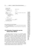
III. Motion in the Gravitational Field of Two Bodies (Satellite
Orbits). The following equations (10) describe the motion of a small body
(a satellite) in the force field of two larger bodies (earth and moon). It is
assumed here that the motion of the three bodies takes place in a fixed plane
and that the two larger bodies rotate with the same constant angular velocity
about their common center of mass and maintain a constant distance to it. In
particular, the effect of the small body on the motion of the two larger bodies
will be ignored (this is the meaning of the adjectives 'small' and 'large'). In
a corotating coordinate system with the center of mass at the origin, the two
larger bodies appear to be at rest. The path of the small body can be described
by a function pair (x(t),y(t)) that satisfies the following system of two second
order differential equations:

(10)

www.pdfgrip.com


6

Introduction

Here the two larger bodies are assumed to lie on the .l:-axis, and the parameter
fJ, respectively fJl, is the ratio of the mass of the body lying on the positive,

respectively negative, x-axis to the combined mass of both bodies. Further, the
unit of length is chosen such that the distance between the two bodies is equal
to 1, and the unit of time such that the angular velocity of the rotation is also
equal to 1 (i.e., a complete revolution lasts 2Jr time units). A closed orbit is
reproduced in the figure. Here fJ :::::; 0.01213, which corresponds to the mass
ratio of the earth-moon system. The initial conditions are

x(O) = 1.2,

y(O)

X(O) = 0,

y(O) :::::; -1.04936.

=

0,

The period T (duration of one complete revolution) is approximately equal to

6.19217.
These examples suggest a variety of problems. First we made use of elementary methods of solution and discovered in the process that for some differential
equations all solutions can be given in closed form (Examples I, II). For differential equations in general, just as in the problem of finding the antiderivative
of an elementary function in integral calculus, the adage holds: Explicit solutions are the exception! The theory of diflerential equations proper has as its
goal a general theory of existence, uniqueness, and other related subjects (for
example, continuous dependence of solutions on various kinds of data) together
with qualitative statements about the behavior of solutions in the large such as
boundedness, oscillation properties, stability, and asymptotic behavior. Theorems about inequalities are also important, as the exercise at the end of this
introduction illustrates.
Several important topics can only be touched briefly in an introductory work
like this one. These include, for instance, the investigation of periodic solutions
to nonlinear differential equations. Periodic solutions have important applications in mechanics (oscillations) and celestial mechanics (closed orbits). However, their mathematical theory is often difficult. Some results in this direction
will be presented in 3.VI-VII and l1.X-XI. For the earth-moon-satellite problem described in III, a special case of the "restricted three-body problem," it was
suggested some time ago that a spaceship on a periodic orbit could be used as a
kind of "bus line" between the earth and the moon. The ensuing investigation
led to the discovery of a new class of periodic orbits; see Arenstorf (1963).
Also, the problem of solving differential equations numerically will not be
treated here. We note that difficult numerical problems arise in connection with
space flight (determining the trajectories of spacecraft). There are efficient numerical algorithms available today that allow the determination and correction
of such trajectories with sufficient accuracy and a tolerable amount of computational effort; see, for instance, the work of Bulirsch and Stoer (1966), from
which the algorithm that produced the above figure is taken.

IV. Exercise. Prove the assertion at the end of Example II. More precisely, show: If s( t) is a positive solution of the differential equation (7) in the
www.pdfgrip.com


Introduction

7

interval a < to :::; t < h (with t j = 00 allowed), s(t) the solution given by (9),
and s(to) = s(to), a < s(to) = v(to) < v(to), then s(t) < s(t) and v(t) < v(t) for
to < t < tj. Further, s(t) is bounded above, and v(t) has one zero (thus, s(t)
describes a return trajectory).
Hint. Derive a differential equation for the difference d(t) = s - sand
conclude from it that d is monotone increasing as long as d is positive. Note
that s < a and v(t) ----+ a as t ----+ 00.

www.pdfgrip.com


Chapter I
First Order Equations:
Some Integrable Cases
§ 1.

Explicit First Order Equations

We consider the explicit first order differential equation

y' = f(x, y).

(1)

The right-hand side f(x, y) of the equation is assumed to be defined as a realvalued function on a set D in the xy-plane.
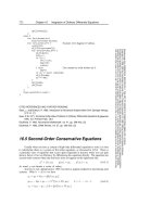
I. Solution. Line Element. Direction Field. Let J be an interval.
(In general, J can be open, closed, half-open, a half-line, or the whole real
line; when special restrictions are necessary, they will be stated explicitly.) A
function y(x) : J ----> IR is called a solution to the differential equation (1) (in J)
if y is differentiable in J, the graph of y is a subset of D, and (1) holds, i.e., if

(x, y(x)) E D

and

y'(x) = f(x, y(x))

y

for all

x E J.

y

I I
I I f
I I I I I
D

I I I I I

/////

Yo

'/////

+----------'------x

+-----------x

Xo

Slope and line element

Direction field

9

www.pdfgrip.com


10

I. First Order Equations: Some Integrable Cases

The differential equation (1) has a simple geometric interpretation. If y(x)
is an integral curve of (1) that passes through a point (xo, Yo) (i.e., y(xo) = Yo),
then the differential equation specifies the slope of the curve at that point:
y/(xo) = f(xo,yo)· This leads naturally to the notions of line element and
direction field, which we will now define. We interpret a numerical triple of the
form (x, y, p) geometrically in the following way: (:r, y) gives a point in the plane,
and the third component p gives the slope of a line through the point (x, y) (ex,
with tan ex = p, is the angle of inclination of the line; see the figure). Such a
triple (or its geometric equivalent) is called a line element. The collection of all
line elements of the form (x, y, f(x, y)), i.e., those with p = f(x, y), is called a
direction .field.
The connection between direction fields and the differential equation (1) can
be expressed in geometric terms as follows: A solution y(x) of a differential

equation "fits" its direction field, i.e., the slope at each point on the solution
curve agrees with the slope of the line element at that point. To put it another
way, if y(x) is a solution in J, then the set of line elements (.T,y(X),y'(x)), with
x E J, is contained in the set of all line elements (x, y, f(x, y)), (:x:, y) E D.
The strategy of sketching a few of the line elements in the direction field and
then trying to draw curves that fit these line elements can be used to get a rough
idea of the nature of the solutions to a differential equation. This procedure
suggests quite naturally the view that for each point (~, 1]) in D there is exactly
one solution curve y(x) passing through that point. A precise formulation of
this idea leads to the notion of

II. The Initial Value Problem. Let a function f(:x:, y), defined on a
set D in the (x,y)-plane, and a fixed point (~,1]) ED be given. A function y(x)
is sought that is differentiable in an interval J with ~ E J such that

y'(x)

y(O

f(x, y(x))
1].

in

J,

(2)

(3)

Equation (3) is called the initial condition. Naturally, in (2) it is assumed that
graphy = {(x,y(x)) :.T E J} cD (otherwise the right-hand side of (2) would
not even be defined).

III. Remarks. (a) D'i.fferential Equations and Families of Curves. The
geometric line of reasoning outlined above can be turned around. Given a family
of curves that completely covers a set D in the plane (precise analytic formulation: a set 111 of differentiable functions whose graphs are pairwise disjoint and
have D as their union), there is a differential equation that has these curves as
its solutions. The right-hand side of this differential equation is determined as
follows: For every (xo, Yo) E D, find the unique function ¢ belonging to M with
¢(xo) = Yo and set f(xo, Yo) = ¢/(xo).
This relationship does not give us very much from the mathematical point of
view. However, it does give an idea of some of the possibilities for the behavior

www.pdfgrip.com


§ 1. Explicit First Order Equations

11

of differential equations, and in addition, it can be used in the construction of
examples.
We will now briefly discuss some mathematical shorthand that is frequently
used.
(b) Sometimes (particularly in examples) when a differential equation is
solved, the function found as the solution is only a solution to the equation on
a subinterval of its domain of definition. When this happens, the expression
"¢J(x) is a solution to the differential equation in the interval J" means that ¢J
is defined at least on J and that the restriction ¢JI J is a solution in the sense of

the definition in I.
(c) If ¢J : J ----> lR is a solution of the differential equation (1) and J' is a
subinterval of J, then, in a trivial way, the restriction 'lj! = ¢JIJI is also a solution
of (1). This is not regarded as a new solution. For instance, the statement "the
differential equation has exactly one solution existing in the interval J" means:
There exists a solution with J as its domain of definition, and every other
solution is a restriction of this solution.
Before giving a detailed investigation of initial value problems, we will study
some simple examples.

I

IV.

y'

= f (x) I

Suppose the function f(x) is continuous in an interval J. Then the set D
is a strip J x lR. The direction field is independent of y. This leads naturally
to the conjecture that all of the solutions can be obtained by translating any
one particular solution in the direction indicated by the y-axis. The analysis
confirms that this guess is true. If ~ E J is fixed, then by the fundamental
theorem of calculus, the function

¢J(x)

:=

l

x

f(t) dt

is a solution of the differential equation satisfying the initial condition y(O
y

,
'
,/
,
,
', /
,
,
,' /
,
,
,' /

,
,

'
,/
,
,

,

,

/"

./

/"

./

/"

./

/"

./

¢J(x)

= 0;

,

"

,

"
"

,
,
,
,

,
,
,
,
,

"
" ,,,
" ,,

./

./

J

X

Direction field in the case where the
right side depends only on x

www.pdfgrip.com

12

1. First Order Equations: Some Integrable Cases

and the general solution can be written in the form
y = y(x;C) = ¢(x)

+ C,

where C is an arbitrary constant. It follows in particular that the initial value
problem (2), (3) has exactly one solution in this case, namely
y(x) = ¢(x)

+ '!].

(4)

The solution exists in all of J.
Note: If J is not compact, then f need not be bounded and as a result may
not be integrable over J. However, since [~, x] is a compact subinterval of J and
f is continuous on [~, .or], the integral in the definition of ¢(x) exists for each
x E J, and the equation ¢' = f holds in all of J.

Example. The equation

y' = x 3

+ cos x

has as solutions

1

.

+ smx + C.

y(x;C) = 4'x 4

If the initial condition is y(l) = 1, then the corresponding solution is
y =

4'1 x 4
+ ·sm x

.

- sm

1

+ 4"3

Thus the problem of finding a solution to a differential equation of type (IV)
is purely a problem in integral calculus-that of finding an antiderivative of a
given function f(x). This motivates a commonly used expression: "Integrating
a differential equation" is synonymous with finding its solutions.

v.

I y'

= g(y)

I

Let g(y) be continuous in an interval J. The direction field here is similar to the one in IV but with the roles of x and y exchanged. This suggests
interchanging x and y and writing the solution curves in the form x = x(y).
A formal calculation gives
dy

-

dx

= g(y)

¢? -

dy

g(y)

= dx

and hence the solution
(5)

If 9 f= 0, then (5) gives a function x = x(y) whose inverse function y(x) is a
solution to the differential equation, as we will show in VII. Finding a solution

www.pdfgrip.com


§ 1. Explicit First Order Equations

13

y

x
Direction field in the case where the
right side depends only on y

that satisfies an initial condition y(~) = TJ involves making a choice of the
constant of integration such that x(TJ) = ~, i.e.,

x(y) = ~

rv

dz

+ iT! g(z)'

(6)

This is a special case of a "differential equation with separable variables." This
type of equation is investigated in more detail in VII. A theorem that will be
proved in that section shows that the initial value problem has exactly one
solution y(x) in a neighborhood of the point ~ if g(TJ) -I- (if g(TJ) -I- 0, then

by continuity 9 -I- in a neighborhood of TJ). This solution can be obtained by
first using formula (6) to get x(y) and then finding the inverse function y(x). If
g(TJ) = 0, then y(x) == TJ is a solution. In this special case, it is quite possible
that there are also other solutions that pass through the point (C TJ), i.e., that
the initial value problem has more than one solution. For more in this regard,
see Example 2 and the discussion in VIII.
The nature of the direction field and the location of the constant of integration in formula (5) suggest that a translation of a solution in the x-direction
will produce another solution: If y(x) is a solution, then so is y(x) := y(x + C).
Indeed, this follows from

°

°

y'(x)

= y'(x + C) = g(y(x + C)) = g(y(x)).

Example 1.
y'

= -2y.

Here D = IR? Using the procedure in (5) one obtains
dy
y

= -2dx ¢} In Iyl = -2x + C

¢}

Iyl = e C - 2x .

The general solution (with ±e c replaced with C) is

y(x; C) = Ce- 2x

(C E lR).

www.pdfgrip.com


14

I. First Order Equations: Some Integrable Cases
y

Solution curves y = Ce- 2x of the
differential equation y' = -2y

The proof that every solution is of this form is elementary: If ¢(x) is any solution
of the differential equation, then

(¢e 2x )' = ¢/e 2x

+ 2¢e 2x

= 0,

i.e., ¢e 2x is a constant. (One could also appeal to the uniqueness statement

proved in VII.) It follows that exactly one solution passes through each point
(~, T/), namely,
y(x; T/e 2 f,) = T/e 2 (f,-x).

Thus we have shown that the initial value problem is uniquely solvable, with a
solution that exists in R

Example 2.
y/ =

v'1YI.

Again D = ]R2. Since the direction field is symmetric, it follows that if y(x) is
a solution, then z(x) = -y( -x) is also a solution. Indeed, we have

z/(.x) = y/( -x) = Jly( -x)1 = ~.
Thus it is sufficient to consider only positive solutions. From (5) it follows that

j Jy
'd

= 2Vfj = x

+ C,

hence
C
y(x; C) = (x +4 )2

in

(-C
)
,00

(C Em.
lTll)

(note that .jfj is positive, whence x > -C, and that for x < -C this formula
does not give a solution to the differential equation). This function gives all of
the positive solutions (this also follows from the uniqueness statement in VII).

www.pdfgrip.com