Fast reliable algorithms for matrices with structure
Bạn đang xem bản rút gọn của tài liệu. Xem và tải ngay bản đầy đủ của tài liệu tại đây (40.41 MB, 356 trang )
www.pdfgrip.com
Fast Reliable Algorithms
for Matrices with Structure
www.pdfgrip.com
This page intentionally left blank
www.pdfgrip.com
Fast Reliable Algorithms
for Matrices with Structure
Edited by
T. Kailath
Stanford University
Stanford, California
A. H. Sayed
University of California
Los Angeles, California
Society for Industrial and Applied Mathematics
Philadelphia
www.pdfgrip.com
Copyright © 1999 by Society for Industrial and Applied Mathematics.
10987654321
All rights reserved. Printed in the United States of America. No part of this book may
be reproduced, stored, or transmitted in any manner without the written permission of
the publisher. For information, write to the Society for Industrial and Applied Mathematics,
3600 University City Science Center, Philadelphia, PA 19104-2688.
Library of Congress Cataloging-in-Publication Data
Fast reliable algorithms for matrices with structure / edited by
T. Kailath, A.M. Sayed
p. cm.
Includes bibliographical references (p. - ) and index.
ISBN 0-89871-431-1 (pbk.)
1. Matrices - Data processing. 2. Algorithms. I. Kailath,
Thomas. II. Sayed, Ali H.
QA188.F38 1999
512.9'434--dc21
99-26368
CIP
rev.
513J1L is a registered trademark.
www.pdfgrip.com
CONTRIBUTORS
Dario A. BINI
Dipartimento di Matematica
Universita di Pisa
Pisa, Italy
Beatrice MEINI
Dipartimento di Matematica
Universita di Pisa
Pisa, Italy
Sheryl BRANHAM
Dept. Math, and Computer Science
Lehman College
City University of New York
New York, NY 10468, USA
Victor Y. PAN
Dept. Math, and Computer Science
Lehman College
City University of New York
New York, NY 10468, USA
Richard P. BRENT
Oxford University Computing Laboratory
Wolfson Building, Parks Road
Oxford OX1 3QD, England
Michael K. NG
Department of Mathematics
The University of Hong Kong
Pokfulam Road, Hong Kong
Raymond H. CHAN
Department of Mathematics
The Chinese University of Hong Kong
Shatin, Hong Kong
Phillip A. REGALIA
Signal and Image Processing Dept.
Inst. National des Telecommunications
F-91011 Evry cedex, France
Shivkumar CHANDRASEKARAN
Dept. Electrical and Computer Engineering
University of California
Santa Barbara, CA 93106, USA
Rhys E. ROSHOLT
Dept. Math, and Computer Science
City University of New York
Lehman College
New York, NY 10468, USA
Patrick DEWILDE
DIMES, POB 5031, 2600GA Delft
Delft University of Technology
Delft, The Netherlands
Ali H. SAVED
Electrical Engineering Department
University of California
Los Angeles, CA 90024, USA
Victor S. GRIGORASCU
Facultatea de Electronica and Telecomunicatii
Universitatea Politehnica Bucuresti
Bucharest, Romania
Paolo TILLI
Scuola Normale Superiore
Piazza Cavalier! 7
56100 Pisa, Italy
Thomas KAILATH
Department of Electrical Engineering
Stanford University
Stanford, CA 94305, USA
Ai-Long ZHENG
Deptartment of Mathematics
City University of New York
New York, NY 10468, USA
v
www.pdfgrip.com
This page intentionally left blank
www.pdfgrip.com
x
Contents
5.3 Iterative Methods for Solving Toeplitz Systems
5.3.1 Preconditioning
5.3.2 Circulant Matrices
5.3.3 Toeplitz Matrix-Vector Multiplication
5.3.4 Circulant Preconditioners
5.4 Band-Toeplitz Preconditioners
5.5 Toeplitz-Circulant Preconditioners
5.6 Preconditioners for Structured Linear Systems
5.6.1 Toeplitz-Like Systems
5.6.2 Toeplitz-Plus-Hankel Systems
5.7 Toeplitz-Plus-Band Systems
5.8 Applications
5.8.1 Linear-Phase Filtering
5.8.2 Numerical Solutions of Biharmonic Equations
5.8.3 Queueing Networks with Batch Arrivals
5.8.4 Image Restorations
5.9 Concluding Remarks
5.A Proof of Theorem 5.3.4
5.B Proof of Theorem 5.6.2
6 ASYMPTOTIC SPECTRAL DISTRIBUTION OF TOEPLITZRELATED MATRICES
Paolo Tilli
6.1 Introduction
6.2 What Is Spectral Distribution?
6.3 Toeplitz Matrices and Shift Invariance
6.3.1 Spectral Distribution of Toeplitz Matrices
6.3.2 Unbounded Generating Function
6.3.3 Eigenvalues in the Non-Hermitian Case
6.3.4 The Szego Formula for Singular Values
6.4 Multilevel Toeplitz Matrices
6.5 Block Toeplitz Matrices
6.6 Combining Block and Multilevel Structure
6.7 Locally Toeplitz Matrices
6.7.1 A Closer Look at Locally Toeplitz Matrices
6.7.2 Spectral Distribution of Locally Toeplitz Sequences
6.8 Concluding Remarks
7 NEWTON'S ITERATION FOR STRUCTURED MATRICES
Victor Y. Pan, Sheryl Branham, Rhys E. Rosholt, and Ai-Long Zheng
7.1 Introduction
7.2 Newton's Iteration for Matrix Inversion
7.3 Some Basic Results on Toeplitz-Like Matrices
7.4 The Newton-Toeplitz Iteration
7.4.1 Bounding the Displacement Rank
7.4.2 Convergence Rate and Computational Complexity
7.4.3 An Approach Using /-Circulant Matrices
7.5 Residual Correction Method
7.5.1 Application to Matrix Inversion
7.5.2 Application to a Linear System of Equations
121
122
123
124
125
130
132
133
133
137
139
140
140
142
144
147
149
150
151
153
153
153
157
158
162
163
164
166
170
174
175
178
182
186
189
189
190
192
194
195
196
198
200
200
201
www.pdfgrip.com
xi
Contents
7.6
7.7
7.A
7.B
7.C
7.5.3 Application to a Toeplitz Linear System of Equations
7.5.4 Estimates for the Convergence Rate
Numerical Experiments
Concluding Remarks
Correctness of Algorithm 7.4.2
Correctness of Algorithm 7.5.1
Correctness of Algorithm 7.5.2
8 FAST ALGORITHMS WITH APPLICATIONS TO MARKOV
CHAINS AND QUEUEING MODELS
Dario A. Bini and Beatrice Meini
8.1 Introduction
8.2 Toeplitz Matrices and Markov Chains
8.2.1 Modeling of Switches and Network Traffic Control
8.2.2 Conditions for Positive Recurrence
8.2.3 Computation of the Probability Invariant Vector
8.3 Exploitation of Structure and Computational Tools
8.3.1 Block Toeplitz Matrices and Block Vector Product
8.3.2 Inversion of Block Triangular Block Toeplitz Matrices
8.3.3 Power Series Arithmetic
8.4 Displacement Structure
8.5 Fast Algorithms
8.5.1 The Fast Ramaswami Formula
8.5.2 A Doubling Algorithm
8.5.3 Cyclic Reduction
8.5.4 Cyclic Reduction for Infinite Systems
8.5.5 Cyclic Reduction for Generalized Hessenberg Systems
8.6 Numerical Experiments
201
203
204
207
208
209
209
211
211
212
214
215
216
217
218
221
223
224
226
227
227
230
234
239
241
9 TENSOR DISPLACEMENT STRUCTURES AND POLYSPECTRAL
MATCHING
245
Victor S. Grigorascu and Phillip A. Regalia
9.1 Introduction
245
9.2 Motivation for Higher-Order Cumulants
245
9.3 Second-Order Displacement Structure
249
9.4 Tucker Product and Cumulant Tensors
251
9.5 Examples of Cumulants and Tensors
254
9.6 Displacement Structure for Tensors
257
9.6.1 Relation to the Polyspectrum
258
9.6.2 The Linear Case
261
9.7 Polyspectral Interpolation
264
9.8 A Schur-Type Algorithm for Tensors
268
9.8.1 Review of the Second-Order Case
268
9.8.2 A Tensor Outer Product
269
9.8.3 Displacement Generators
272
9.9 Concluding Remarks
275
www.pdfgrip.com
xii
Contents
10 MINIMAL COMPLEXITY REALIZATION OF STRUCTURED
MATRICES
277
Patrick Dewilde
10.1 Introduction
277
10.2 Motivation of Minimal Complexity Representations
278
10.3 Displacement Structure
279
10.4 Realization Theory for Matrices
280
10.4.1 Nerode Equivalence and Natural State Spaces
283
10.4.2 Algorithm for Finding a Realization
283
10.5 Realization of Low Displacement Rank Matrices
286
10.6 A Realization for the Cholesky Factor
289
10.7 Discussion
293
A USEFUL MATRIX RESULTS
Thomas Kailath and Ali H. Sayed
A.I Some Matrix Identities
A.2 The Gram-Schmidt Procedure and the QR Decomposition
A.3 Matrix Norms
A.4 Unitary and ./-Unitary Transformations
A.5 Two Additional Results
297
B ELEMENTARY TRANSFORMATIONS
Thomas Kailath and Ali H. Sayed
B.I Elementary Householder Transformations
B.2 Elementary Circular or Givens Rotations
B.3 Hyperbolic Transformations
309
BIBLIOGRAPHY
321
INDEX
339
298
303
304
305
306
310
312
314
www.pdfgrip.com
PREFACE
The design of fast and numerically reliable algorithms for large-scale matrix problems
with structure has become an increasingly important activity, especially in recent years,
driven by the ever-increasing complexity of applications arising in control, communications, computation, and signal processing.
The major challenge in this area is to develop algorithms that blend speed and numerical accuracy. These two requirements often have been regarded as competitive, so
much so that the design of fast and numerically reliable algorithms for large-scale structured linear matrix equations has remained a significant open issue in many instances.
This problem, however, has been receiving increasing attention recently, as witnessed
by a series of international meetings held in the last three years in Santa Barbara (USA,
Aug. 1996), Cortona (Italy, Sept. 1996), and St. Emilion (Prance, Aug. 1997). These
meetings provided a forum for the exchange of ideas on current developments, trends,
and issues in fast and reliable computing among peer research groups. The idea of this
book project grew out of these meetings, and the chapters are selections from works
presented at the meetings. In the process, several difficult decisions had to be made;
the editors beg the indulgence of participants whose contributions could not be included
here.
Browsing through the chapters, the reader soon will realize that this project is
unlike most edited volumes. The book is not merely a collection of submitted articles;
considerable effort went into blending the several chapters into a reasonably consistent
presentation. We asked each author to provide a contribution with a significant tutorial
value. In this way, the chapters not only provide the reader with an opportunity to
review some of the most recent advances in a particular area of research, but they do
so with enough background material to put the work into proper context. Next, we
carefully revised and revised again each submission to try to improve both clarity and
uniformity of presentation. This was a substantial undertaking since we often needed to
change symbols across chapters, to add cross-references to other chapters and sections,
to reorganize sections, to reduce redundancy, and to try to state theorems, lemmas, and
algorithms uniformly across the chapters. We did our best to ensure a uniformity of
presentation and notation but, of course, errors and omissions may still exist and we
apologize in advance for any of these. We also take this opportunity to thank the authors
for their patience and for their collaboration during this time-consuming process. In
all we believe the book includes a valuable collection of chapters that cover in some
detail different aspects of the most recent trends in the theory of fast algorithms, with
emphasis on implementation and application issues.
The book may be divided into four distinct parts:
1. The first four chapters deal with fast direct methods for the triangular factorization
xiii
www.pdfgrip.com
xiv
Preface
of structured matrices, as well as the solution of structured linear systems of
equations. The emphasis here is mostly on the generalized Schur algorithm, its
numerical properties, and modifications to ensure numerical stability.
2. Chapters 5, 6, and 7 deal with fast iterative methods for the solution of structured
linear systems of equations. The emphasis here is on the preconditioned conjugate
gradient method and on Newton's method.
3. Chapters 8 to 10 deal with extensions of the notion of structure to the block
case, the tensor case, and to the input-output framework. Chapter 8 presents
fast algorithms for block Toeplitz systems of equations and considers applications
in Markov chains and queueing theory. Chapter 9 studies tensor displacement
structure and applications in polyspectral interpolation. Chapter 10 discusses
realization theory and computational models for structured problems.
4. We have included two appendices that collect several useful matrix results that
are used in several places in the book.
Acknowledgments. We gratefully acknowledge the support of the Army Research Office and the National Science Foundation in funding the organization of the Santa Barbara Workshop. Other grants from these agencies, as well as from the Defense Advanced
Research Projects Agency and the Air Force Office of Scientific Research, supported the
efforts of the editors on this project. We are also grateful to Professors Alan Laub of
University of California Davis and Shivkumar Chandrasekaran of University of California Santa Barbara for their support and joint organization with the editors of the 1996
Santa Barbara Workshop. It is also a pleasure to thank Professors M. Najim of the
University of Bordeaux and P. Dewilde of Delft University, for their leading role in the
St. Emilion Workshop, and Professor D. Bini of the University of Pisa and several of
his Italian colleagues, for the fine 1996 Toeplitz Workshop in Cortona.
October 1998
T. Kailath
Stanford, CA
A. H. Sayed
Westwood, CA
www.pdfgrip.com
NOTATION
N
Z
R
C
0
The
The
The
The
The
C-2-n
The set of 27r-periodic complex-valued continuous
functions defined on [—7r,7r].
The set of complex-valued continuous functions
with bounded support in R.
The set of bounded and uniformly continuous
complex-valued functions over R.
Co(M)
Cb(R)
•T
•*
a = b
col{a, 6}
diag{a, 6}
tridiag{a, 6, c}
a0 6
1
\x]
[x\
0
In
£(x)
<C>
set of natural numbers.
set of integer numbers.
set of real numbers.
set of complex numbers.
empty set.
Matrix transposition.
Complex conjugation for scalars and conjugate
transposition for matrices.
The quantity a is defined as b.
A column vector with entries a and b.
A diagonal matrix with diagonal entries a and b.
A tridiagonal Toeplitz matrix with b along its diagonal,
a along its lower diagonal, and c along its upper diagonal,
The same as diag{a, b}.
v^
The smallest integer ra > x.
The largest integer m < x.
A zero scalar, vector, or matrix.
The identify matrix of size n x n.
A lower triangular Toeplitz matrix whose first column is x.
The end of a proof, an example, or a remark.
XV
www.pdfgrip.com
xvi
Notation
|| • || 2
|| • ||i
|| • 11 oo
|| • ||p
|| • ||
\A\
\i(A)
(7i(A)
K(A)
coudk(A)
e
O(n)
On(e)
~
7
CG
LDU
PCG
QR
The Euclidean norm of a vector or the maximum
singular value of a matrix.
The sum of the absolute values of the entries of a
vector or the maximum absolute column sum of a matrix.
The largest absolute entry of a vector or the maximum
absolute row sum of a matrix.
The Probenius norm of a matrix.
Some vector or matrix norm.
A matrix with elements \a,ij\.
ith eigenvalue of A.
ith singular value of A.
Condition number of a matrix A, given by HA^H-A" 1 !^.
Equal to H^llfcllA- 1 ^.
Machine precision.
A constant multiple of n, or of the order of n.
O(ec(n)}, where c(n) is some polynomial in n.
A computed quantity in a finite precision algorithm.
An intermediate exact quantity in a finite precision algorithm.
The
The
The
The
conjugate gradient method.
lower-diagonal-upper triangular factorization of a matrix.
preconditioned conjugate gradient method.
QR factorization of a matrix.
www.pdfgrip.com
Chapter 1
DISPLACEMENT STRUCTURE
AND ARRAY ALGORITHMS
Thomas Kailath
1.1
INTRODUCTION
Many problems in engineering and applied mathematics ultimately require the solution of n x n linear systems of equations. For small-size problems, there is often
not much else to do except to use one of the already standard methods of solution
such as Gaussian elimination. However, in many applications, n can be very large
(n ~ 1000, n ~ 1,000,000) and, moreover, the linear equations may have to be solved
over and over again, with different problem or model parameters, until a satisfactory
solution to the original physical problem is obtained. In such cases, the O(n3) burden,
i.e., the number of flops required to solve an n x n linear system of equations, can become
prohibitively large. This is one reason why one seeks in various classes of applications
to identify special or characteristic structures that may be assumed in order to reduce
the computational burden. Of course, there are several different kinds of structure.
A special form of structure, which already has a rich literature, is sparsity; i.e.,
the coefficient matrices have only a few nonzero entries. We shall not consider this
already well studied kind of structure here. Our focus will be on problems, as generally
encountered in communications, control, optimization, and signal processing, where the
matrices are not sparse but can be very large. In such problems one seeks further
assumptions that impose particular patterns among the matrix entries. Among such
assumptions (and we emphasize that they are always assumptions) are properties such
as time-invariance, homogeneity, stationarity, and rationality, which lead to familiar
matrix structures, such as Toeplitz, Hankel, Vandermonde, Cauchy, Pick, etc. Several
fast algorithms have been devised over the years to exploit these special structures. The
numerical (accuracy and stability) properties of several of these algorithms also have
been studied, although, as we shall see from the chapters in this volume, the subject is by
no means closed even for such familiar objects as Toeplitz and Vandermonde matrices.
In this book, we seek to broaden the above universe of discourse by noting that even
more common than the explicit matrix structures, noted above, are matrices in which
the structure is implicit. For example, in least-squares problems one often encounters
products of Toeplitz matrices; these products generally are not Toeplitz, but on the other
hand they are not "unstructured." Similarly, in probabilistic calculations the matrix of
interest often is not a Toeplitz covariance matrix, but rather its inverse, which is rarely
1
www.pdfgrip.com
2
Displacement Structure and Array Algorithms
Chapter 1
Toeplitz itself, but of course is not unstructured: its inverse is Toeplitz. It is well known
that O(n2) flops suffice to solve linear systems with an n x n Toeplitz coefficient matrix;
a question is whether we will need O(n3) flops to invert a non-Toeplitz coefficient matrix
whose inverse is known to be Toeplitz. When pressed, one's response clearly must be
that it is conceivable that O(n 2 ) flops will suffice, and we shall show that this is in fact
true.
Such problems, and several others that we shall encounter in later chapters, suggest the need for a quantitative way of defining and identifying structure in (dense)
matrices. Over the years we have found that an elegant and useful way is the concept of displacement structure. This has been useful for a host of problems apparently
far removed from the solution of linear equations, such as the study of constrained and
unconstrained rational interpolation, maximum entropy extension, signal detection, system identification, digital filter design, nonlinear Riccati differential equations, inverse
scattering, certain Fredholm and Wiener-Hopf integral equations, etc. However, in this
book we shall focus attention largely on displacement structure in matrix computations.
For more general earlier reviews, we may refer to [KVM78], [Kai86], [Kai91], [HR84],
[KS95a].
1.2
TOEPLITZ MATRICES
The concept of displacement structure is perhaps best introduced by considering the
much-studied special case of a Hermitian Toeplitz matrix,
The matrix T has constant entries along its diagonals and, hence, it depends only on
n parameters rather than n2. As stated above, it is therefore not surprising that many
matrix problems involving T, such as triangular factorization, orthogonalization, and
inversion, have solution complexity O(n2) rather than O(n3) operations. The issue is
the complexity of such problems for inverses, products, and related combinations of
Toeplitz matrices such as r-1,TiT2,Ti - T2T^1T^ (TiT2)~lT3 .... As mentioned earlier, although these are not Toeplitz, they are certainly structured and the complexity
of inversion and factorization may be expected to be not much different from that for
a pure Toeplitz matrix, T. It turns out that the appropriate common property of all
these matrices is not their "Toeplitzness," but the fact that they all have (low) displacement rank in a sense first defined in [KKM79a], [KKM79b] and later much studied and
generalized. When the displacement rank is r, r < n, the solution complexity of the
above problems turns out to be O(rn 2 ). Now for some formal definitions.
The displacement of a Hermitian matrix R = [^"J^o € C nxn was originally1
defined in [KKM79a], [KKM79b] as
1
Other definitions will be introduced later. We may note that the concept was first identified in
studying integral equations (see, e.g., [KLM78]).
www.pdfgrip.com
Section 1.2. Toeplitz Matrices
3
where * denotes Hermitian conjugation (complex conjugation for scalars) and Z is the
n x n lower shift matrix with ones on the first subdiagonal and zeros elsewhere,
The product ZRZ* then corresponds to shifting R downward along the main diagonal
by one position, explaining the name displacement for VzR~ The situation is depicted
in Fig. 1.1.
Figure 1.1. VzR is obtained by shifting R downward along the diagonal.
If V z R has (low) rank, say, r, independent of n, then R is said to be structured
with respect to the displacement V^ defined by (1.2.2), and r is called the displacement
rank of R. The definition can be extended to non-Hermitian matrices, and this will be
briefly described later. Here we may note that in the Hermitian case, V^jR is Hermitian
and therefore has further structure: its eigenvalues are real and so we can define the
displacement inertia of R as the pair {p, q}, where p (respectively, q) is the number of
strictly positive (respectively, negative) eigenvalues of V^-R. Of course, the displacement
rank is r = p -f q- Therefore, we can write
where J = J* = (Ip@—Iq) is a signature matrix and G e C n x r . The pair [G, J} is called
a Vz-generator of R. This representation is clearly not unique; for example, {G0, J}
is also a generator for any J-unitary matrix B (i.e., for any 6 such that 9JO* = J).
This is because
Nonminimal generators (where G has more than r columns) are sometimes useful, although we shall not consider them here.
Returning to the Toeplitz matrix (1.2.1), it is easy to see that T has displacement rank 2, except when all Ci, i ^ 0, are zero, a case we shall exclude. Assuming
www.pdfgrip.com
4
Displacement Structure and Array Algorithms
Chapter 1
CQ = 1, a generator for T is {:co,yo,(l © —!)}> where rro = col{l,ci,... ,c n _i} and
yQ = col{0, c i , . . . , c n _i} (the notation col{-} denotes a column vector with the specified
entries):
It will be shown later that if we define T# = IT 1I, where / denotes the reversed
identity with ones on the reversed diagonal and zeros elsewhere, then T# also has Vzdisplacement inertia {!,!}• The product T\T<2 of two Toeplitz matrices, which may
not be Hermitian, will be shown to have displacement rank < 4. The significance of
displacement rank with respect to the solution of linear equations is that the complexity
can be reduced to O(rn2) from O(n3).
The well-known Levinson algorithm [Lev47] is one illustration of this fact. The bestknown form of this algorithm (independently obtained by Durbin [Dur59]) refers to the
so-called Yule-Walker system of equations
where an = [ an,n an,n-i ããã ôn,iằl ] and cr2 are the (n + 1) unknowns and Tn
is a positive-definite (n + 1) x (n + 1) Toeplitz matrix. The easily derived and now
well-known recursions for the solution are
where
and
The above recursions are closely related to certain (nonrecursive2) formulas given by
Szego [Sze39] and Geronimus [Ger54] for polynomials orthogonal on the unit circle,
as discussed in some detail in [KaiQl]. It is easy to check that the {7*} are all less
than one in magnitude; in signal processing applications, they are often called reflection
coefficients (see, e.g., [Kai85], [Kai86]).
While the Levinson-Durbin algorithm is widely used, it has limitations for certain
applications. For one thing, it requires the formation of inner products and therefore
is not efficiently parallelizable, requiring O(nlogn) rather than O(n) flops, with O(n)
processors. Second, while it can be extended to indefinite and even non-Hermitian
Toeplitz matrices, it is difficult to extend it to non-Toeplitz matrices having displacement structure. Another problem is numerical. An error analysis of the algorithm in
[CybSO] showed that in the case of positive reflection coefficients {7*}, the residual error produced by the Levinson-Durbin procedure is comparable to the error produced
2
They defined 7» as — ai+i,»+i.
www.pdfgrip.com
Section 1.2.
Toeplitz Matrices
5
by the numerically well-behaved Cholesky factorization [GV96, p. 191]. Thus in this
special case the Levinson-Durbin algorithm is what is called weakly stable, in the sense
of [Bun85], [Bun87]—see Sec. 4.2 of this book. No stability results seem to be available
for the Levinson-Durbin algorithm for Toeplitz matrices with general {7i}.
To motivate an alternative (parallelizable and stable) approach to the problem, we
first show that the Levinson-Durbin algorithm directly yields a (fast) triangular factorization of T~l. To show this, note that stacking the successive solutions of the
Yule-Walker equations (1.2.6) in a lower triangular matrix yields the equality
which, using the Hermitian nature of T, yields the unique triangular factorization of
the inverse of Tn:
where Dn = diag{crg,a\,...,a^}.
However, it is a fact, borne out by results in many different problems, that ultimately
even for the solution of linear equations the (direct) triangular factorization of T rather
than T~l is more fundamental. Such insights can be traced back to the celebrated
Wiener-Hopf technique [WH31] but, as perhaps first noted by Von Neumann and by
Turing (see, e.g., [Ste73]), direct factorization is the key feature of the fundamental
Gaussian elimination method for solving linear equations and was effectively noted as
such by Gauss himself (though of course not in matrix notation).
Now a fast direct factorization of Tn cannot be obtained merely by inverting the
factorization (1.2.10) of T~l, because that will require O(n3) flops. The first fast algorithm was given by Schur [Schl7], although this fact was realized only much later in
[DVK78]. In the meantime, a closely related direct factorization algorithm was derived
by Bareiss [Bar69], and this is the designation used in the numerical analysis community. Morf [Mor70], [Mor74], Rissanen [Ris73], and LeRoux-Gueguen [LG77] also made
independent rediscoveries.
We shall show in Sec. 1.7.7 that the Schur algorithm can also be applied to solve
Toeplitz linear equations, at the cost of about 30% more computations than via the
Levinson-Durbin algorithm. However, in return we can compute the reflection coefficients without using inner products, the algorithm has better numerical properties
www.pdfgrip.com
6
Displacement Structure and Array Algorithms
Chapter 1
(see Chs. 2-4 and also [BBHS95], [CS96]), and as we shall show below, it can be elegantly and usefully extended by exploiting the concept of displacement structure. These
generalizations are helpful in solving the many classes of problems (e.g., interpolation)
mentioned earlier (at the end of Sec. 1.1). Therefore, our major focus in this chapter
will be on what we have called generalized Schur algorithms.
First, however, let us make a few more observations on displacement structure.
1.3
VERSIONS OF DISPLACEMENT STRUCTURE
There are of course other kinds of displacement structure than those introduced in
Sec. 1.2, as already noted in [KKM79a]. For example, it can be checked that
where Z-\ denotes the circulant matrix with first row [ 0 ... 0 — 1 ]. This fact has
been used by Heinig [Hei95] and by [GKO95] to obtain alternatives to the LevinsonDurbin and Schur algorithms for solving Toeplitz systems of linear equations, as will
be discussed later in this chapter (Sec. 1.13). However, a critical point is that because
Z_i is not triangular, these methods apply only to fixed n, and the whole solution has
to be repeated if the size is increased even by one. Since many applications in communications, control, and signal processing involve continuing streams of data, recursive
triangular factorization is often a critical requirement. It can be shown [LK86] that such
factorization requires that triangular matrices be used in the definition of displacement
structure, which is what we shall do henceforth.
One of the first extensions of definition (1.2.2) was to consider
where, for reasons mentioned above, F is a lower triangular matrix; see [LK84], [CKL87].
One motivation for such extensions will be seen in Sec. 1.8. Another is that one can
include matrices such as Vandermonde, Cauchy, Pick, etc. For example, consider the
so-called Pick matrix, which occurs in the study of analytic interpolation problems,
where {iii,t>i} are row vectors of dimensions p and q, respectively, and fi are complex
points inside the open unit disc (|/$| < 1). If we let F denote the diagonal matrix
diag{/o, /i,..., /n-i}, then it can be verified that P has displacement rank (p + q) with
respect to F since
In general, one can write for Hermitian R € C n x n ,
for some triangular F € C n x n , a signature matrix J = (Ip © -Iq] e C r x r , and
G e C nxr , with r independent of n. The pair {G, J} will be called a V^-generator
www.pdfgrip.com
Section 1.3. Versions of Displacement Structure
7
of R. Because Toeplitz and, as we shall see later, several Toeplitz-related matrices are
best studied via this definition, matrices with low V^-displacement rank will be called
Toeplitz-like. However, this is strictly a matter of convenience.
We can also consider non-Hermitian matrices R, in which case the displacement can
hp HpfinpH as
where F and A are n x n lower triangular matrices. In some cases, F and A may
coincide—see (1.3.7) below. When Vp,AR has low rank, say, r, we can factor it
(nonuniquely) as
where G and B are also called generator matrices,
One particular example is the case of a non-Hermitian Toeplitz matrix T = [cj_j]™ ._0 ,
which can be seen to satisfy
This is a special case of (1.3.6) with F = A = Z.
A second example is a Vandermonde matrix,
which can be seen to satisfy
where F is now the diagonal matrix F = diag {cti,..., an}.
Another common form of displacement structure, first introduced by Heinig and
Rost [HR84], is what we call, again strictly for convenience, a Hankel-like structure. We
shall say that a matrix R € C n x n is Hankel-like if it satisfies a displacement equation
of the form
for some lower triangular F e C nxn and A e C n x n , and generator matrices G
to express the displacement equation as
www.pdfgrip.com
8
Displacement Structure and Array Algorithms
Chapter 1
for some generator matrix G € C n x r and signature matrix J that satisfies J = J* and
J2 = 7. To avoid a notation explosion, we shall occasionally use the notation Vp,AR
for both Toeplitz-like and Hankel-like structures.
As an illustration, consider a Hankel matrix, which is a symmetric matrix with real
constant entries along the antidiagonals,
It can be verified that the difference ZH — HZ* has rank 2 since
(1.3.13)
We therefore say that H has displacement rank 2 with respect to the displacement
operation (1.3.11) with F = iZ and J as above. Here, i = \/~l and is introduced in
order to obtain a J that satisfies the normalization conditions J = J*, J2 = /.
A problem that arises here is that H cannot be fully recovered from its displacement
representation, because the entries {/in-i, • - - , ^2n-2J do not appear in (1.3.14). This
"difficulty" can be accommodated in various ways (see, e.g., [CK91b], [HR84], [KS95a]).
One way is to border H with zeros and then form the displacement, which will now have
rank 4. Another method is to form the 2n x In (triangular) Hankel matrix with top
row {/IQ, ..., /i2n-i}; now the displacement rank will be two; however, note that in both
cases the generators have the same number of entries. In general, the problem is that
the displacement equation does not have a unique solution. This will happen when the
displacement operator in (1.3.3)-(1.3.6) or (1.3.10)-(1.3.11) has a nontrivial nullspace
or kernel. In this case, the generator has to be supplemented by some additional information, which varies from case to case. A detailed discussion, with several examples, is
given in [KO96], [KO98].
Other examples of Hankel-like structures include Loewner matrices, Cauchy matrices, and Cauchy-like matrices, encountered, for example, in the study of unconstrained
rational interpolation problems (see, e.g., [AA86], [Fie85], [Vav91]). The entries of an
n x n Cauchy-like matrix R have the form
www.pdfgrip.com
Section 1.3.
Versions of Displacement Structure
9
where Ui and Vj denote 1 xr row vectors and the {/$, a,i} are scalars. The Loewner matrix
is a special Cauchy-like matrix that corresponds to the choices r = 2, HI — [ fa 1 ],
and V{ = \ 1 — Ki ], and, consequently, u^ = fa — & :
Cauchy matrices, on the other hand, arise from the choices r = 1 and u^ = 1 = Vi :
It is easy to verify that a Cauchy-like matrix is Hankel-like since it satisfies a displacement equation of the form
where F and A are diagonal matrices:
F = diagonal {/ 0 ,..., /n-i}, A = diagonal {a 0 ,..., a n _i}.
Hence, Loewner and Cauchy matrices are also Hankel-like. Another simple example is
the Vandermonde matrix (1.3.8) itself, since it satisfies not only (1.3.9) but also
where A is the diagonal matrix (assuming ai ^ 0)
Clearly, the distinction between Toeplitz-like and Hankel-like structures is not very
tight, since many matrices can have both kinds of structure including Toeplitz matrices
themselves (cf. (1.2.5) and (1.3.1)).
Toeplitz- and Hankel-like structures can be regarded as special cases of the generalized displacement structure [KS91], [Say92], [SK95a], [KS95a]:
where {fi,A,F, A} are n x n and {(7, B} are n x r. Such equations uniquely define
R when the diagonal entries {ui,Si,fi,di} of the displacement operators {fi,A,F, A}
satisfy
This explains the difficulty we had in the Hankel case, where the diagonal entries of
F = A = Z in (1.3.14) violate the above condition. The restriction that {£), A, F, A}
are lower triangular is the most general one that allows recursive triangular factorization
(cf. a result in [LK86]). As mentioned earlier, since this is a critical feature in most of
our applications, we shall assume this henceforth.
www.pdfgrip.com
10
Displacement Structure and Array Algorithms
Chapter 1
The Generating Function Formulation
We may remark that when {Q, A, F, A} are lower triangular Toeplitz, we can use generating function notation—see [LK84], [LK86]; these can be extended to more general
{rfc,A,F, A} by using divided difference matrices—see [Lev83], [Lev97]. The generating function formulation enables connections to be made with complex function theory
and especially with the extensive theory of reproducing kernel Hilbert spaces of entire
functions (deBranges spaces)—see, e.g., [AD86], [Dym89b], [AD92].
Let us briefly illustrate this for the special cases of Toeplitz and Hankel matrices,
T = [ci-j], H = [hi+j]. To use the generating function language, we assume that the
matrices are semi-infinite, i.e., i,j 6 [0, oo). Then straightforward calculation will yield,
assuming CQ == 1, the expression
where c(z) is (a so-called Caratheodory function)
The expression can also be rewritten as
where
In the Hankel case, we can write
where
and
Generalizations can be obtained by using more complex (G(-), J} matrices and with
However, to admit recursive triangular factorization, one must asume that d(z, w) has
the form (see [LK86])
www.pdfgrip.com
Section 1.3.
Versions of Displacement Structure
11
for some {a(.z),b(z)}. The choice of d(z,w) also has a geometric significance. For
example, di(z, w} partitions the complex plane with respect to the unit circle, as follows:
Similarly, 6^2(2, w) partitions the plane with respect to the real axis. If we used ^3(2, w) =
z -f w*, we would partition the plane with respect to the imaginary axis.
We may also note that the matrix forms of
will be, in an obvious notation,
while using d-2(z,w] it will be
Here, Z denotes the semi-infinite lower triangular shift matrix. Likewise, {7£, denote semi-infinite matrices.
We shall not pursue the generating function descriptions further here. They are
useful, inter alia, for studying root distribution problems (see, e.g., [LBK91]) and, as
mentioned above, for making connections with the mathematical literature, especially
the Russian school of operator theory. A minor reason for introducing these descriptions
here is that they further highlight connections between displacement structure theory
and the study of discrete-time and continuous-time systems, as we now explain briefly.
Lyapunov, Stein, and Displacement Equations
When J = /, (1.3.19) and (1.3.20) are the discrete-time and continuous-time Lyapunov
equations much studied in system theory, where the association between discrete-time
systems and the unit circle and continuous-time systems and half-planes, is well known.
There are also well-known transformations (see [KaiSO, p. 180])between discrete-time
and continuous-time (state-space) systems, so that in principle all results for Toeplitzlike displacement operators can be converted into the appropriate results for Hankel-like
operators. This is one reason that we shall largely restrict ourselves here to the Toeplitzlike Hermitian structure (1.3.3); more general results can be found in [KS95a].
A further remark is that equations of the form (1.3.10), but with general right sides,
are sometimes called Sylvester equations, while those of the form (1.3.6) are called Stein
equations. For our studies, low-rank factorizations of the right side as in (1.3.10) and
(1.3.6) and especially (1.3.11) and (1.3.3) are critical (as we shall illustrate immediately),
which is why we call these special forms displacement equations.
Finally, as we shall briefly note in Sec. 1.14.1, there is an even more general version of
displacement theory applying to "time-variant" matrices (see, e.g., [SCK94], [SLK94b],
[CSK95]). These extensions are useful, for example, in adaptive filtering applications
and also in matrix completion problems and interpolation problems, where matrices
change with time but in such a way that certain displacement differences undergo only
low-rank variations.
A Summary
To summarize, there are several ways to characterize the structure of a matrix, using for
example (1.3.6), (1.3.10), or (1.3.16). However, in all cases, the main idea is to describe