Coordinate geometry
Bạn đang xem bản rút gọn của tài liệu. Xem và tải ngay bản đầy đủ của tài liệu tại đây (11.8 MB, 337 trang )
www.pdfgrip.com
COORDINATE
GEOMETRY
BY
LUTHER PFAHLER EISENHART
PROFESSOR OF MATHEMATICS
PRINCETON UNIVERSITY
DOVER PUBLICATIONS, INC.
NEW YORK NEW YORK
www.pdfgrip.com
Copyright, 1939, by Ginn and
Company
All Rights Reserved
This new Dover edition
is
first
published in 1960
an unabridged and unaltered republication
of the First Edition.
book is republished by permission of
Ginn and Company, the original publisher of
This
this text.
Manufactured
in the
United States of America
Dover Publications, Inc.
180 Varick Street
New York
14,
New York
www.pdfgrip.com
Preface
The purposes and
general plan of this
book are
set forth
a text has been tested
and proved through use during two years in freshman courses
in Princeton University. Each year it has been revised as a
result of suggestions not only by the members of the staff but
also by the students, who have shown keen interest and helpfulness in the development of the project.
An unusual feature of the book is the presentation of coordinate geometry in the plane in such manner as to lead readily
to the study of lines and planes in space as a generalization of the
geometry of the plane this is done in Chapter 2. It has been
our experience that the students have little, if any, difficulty in
handling the geometry of space thus early in the course, in the
in the Introduction.
Its practicability as
;
which it is developed in this chapter.
have
also found that students who have studied deterWe
minants in an advanced course in algebra find for the first time
in the definition and frequent use of determinants in this book
an appreciation of the value and significance of this subject.
In the preparation and revisions of the text the author has
received valuable assistance from the members of the staff at
in particular, Professors Knebelman and Tucker
Princeton
Messrs.
and
Tompkins, Daly, Fox, Titt, Traber, Battin, and
Johnson the last two have been notably helpful in the preparation of the final form of the text and in the reading of the
proof. The Appendix to Chapter 1, which presents the relation
between the algebraic foundations of coordinate geometry and
axioms of Hilbert for Euclidean plane geometry, is due in the
main to Professors Bochner and Church and Dr. Tompkins,
particularly to the latter, at whose suggestion it was prepared
and incorporated. The figures were drawn by Mr. J. H. Lewis.
It remains for me to express my appreciation of the courtesy
and cooperation of Ginn and Company in the publication of
way
in
;
this book.
LUTHER PFAHLER EISENHART
iii
www.pdfgrip.com
www.pdfgrip.com
Contents
PAGE
INTRODUCTION
ix
CHAPTER
Points
and Lines
1
in tKe
Plane
SECTION
1.
The Equation
2.
Cartesian Coordinates in the Plane
3.
of the First Degree in x
Distance between
rection Cosines
Internal
5.
An Equation
8
Direction
of a Line
Two
Direction Cosines of a Line
20
Angle
Lines
27
of a Line
33
The Slope
8.
Directed Distance from a Line to a Point
Two
11
17
Parametric Equations of a Line
7.
9.
Numbers and Di-
Angle between Directed Line Segments
Numbers and
Direction
between
Points
3
and External Division of a Line Segment
4.
6.
Two
and y
Equations of the First Degree in x and y
35
-
Determinants
of the Second Order
39
10.
The Set
47
11.
Oblique Axes
53
12.
The
54
13.
Resume
of Lines through a Point
Circle
Line Coordinates
CHAPTER
Lines and Planes in Space
14.
15.
62
2
Determinants
Rectangular Coordinates in Space
71
Two
Points
Distance between
Direction Numbers and Direction Cosines of a Line Segment Angle between Two Line
Segments
76
www.pdfgrip.com
Contents
PAGE
SECTION
Equations of a Line Direction Numbers and Direction Cosines of a Line Angle of Two Lines
82
17.
An Equation
88
18.
The Directed Distance from a Plane
16.
of a Plane
to a Point
The
Dis-
tance from a Line to a Point
95
Two
19.
Equations of the First Degree in Three
Line as the Intersection of Two Planes
20.
Two Homogeneous
Unknowns A
98
Equations of the First Degree in Three
Unknowns
21.
104
Determinants of the Third Order
Degree in Three Unknowns
Three Equations of the
106
First
22.
23.
Three Homogeneous Equations of the First Degree
in
Three
Unknowns
114
Equations of Planes Determined by Certain Geometric ConShortest Distance between Two Lines
119
The Configurations
123
ditions
24.
of Three Planes
25. Miscellaneous Exercises
26.
Determinants of
27. Solution of
of
The Sphere
127
130
Any Order
Equations of the First Degree
of Four Dimensions
in
Any Number
Unknowns Space
CHAPTER
137
5
Transformations of Coordinates
28.
Transformations of Rectangular Coordinates
29. Polar Coordinates in the Plane
30.
Transformations of Rectangular Coordinates in Space
31. Spherical
and Cylindrical Coordinates
vi
149
154
160
166
www.pdfgrip.com
Contents
CHAPTER
4
The Conies Locus Problems
PAGE
171
SECTION
32.
A Geometric
33.
The Parabola
174
34.
Tangents and Polars
177
35. Ellipses
36.
Definition of the Conies
and Hyperbolas
182
Conjugate Diameters and Tangents of Central Conies
The Asymptotes
37. Similar Central Conies
191
of a Hyperbola
196
Conjugate Hyperbolas
38.
The Conies
39.
Equations of Conies
ordinate Axes
as Plane Sections of a Right Circular
Whose Axes Are
40.
The General Equation
41.
The Determination
Form
Cone
^Parallel to the
201
Co203
of the Second Degree
Invariants
of a Conic from Its Equation in General
215
42. Center, Principal Axes,
and Tangents of a Conic Defined
by a General Equation
43.
208
221
Locus Problems
229
ti
CHAPTER
The Quadric
44. Surfaces of Revolution
45. Canonical
46.
5
Surfaces
The Quadric
Surfaces of Revolution
Equations of the Quadric Surfaces
243
The Ruled Quadrics
47. Quadrics
Whose
248
Principal Planes
Are
Parallel to the
Co252
ordinate Planes
48.
239
The General Equation of the Second Degree in x, y, and z
The Characteristic Equation Tangent Planes to a Quadric
vii
256
www.pdfgrip.com
Contents
PAGE
SECTION
49. Centers
50.
The
Vertices
Invariants
Points of
7, /,
51. Classification of the
D, and
Symmetry
A
267
271
Quadrics
APPENDIX TO CHAPTER
INDEX
264
279
1
293
Vlll
www.pdfgrip.com
Introduction
Coordinate geometry is so called because it uses in the treatof geometric problems a system of coordinates, which
associates with each point of a geometric figure a set of numso that the conditions which each point
coordinates
bers
ment
satisfy are expressible by means of equations or inequaliordinarily involving algebraic quantities and at times
trigonometric functions. By this means a geometric problem is
must
ties
reduced to an algebraic problem, which most people can handle
with greater ease and confidence. After the algebraic solution
has been obtained, however, there, remains its geometric interpretation to be determined for^ttigdPfpblem is geometric, and
4
algebra is a means to its solution, not the end. This method
was introduced by Rene Descartes in La Geometric, published
in 1636
accordingly coordinate geometry is sometimes called
Cartesian geometry. Before the time of Descartes geometric
reasoning only was used in the study of geometry. The advance
in the development of geometric ideas since the time of Descartes
is largely due to the introduction of his method.
Geometry deals with spatial concepts. The problems of
physics, astronomy, engineering, etc. involve not only space but
usually time also. The method of attack upon these problems
is similar to that used in coordinate geometry.
However,
geometric problems, because of the absence of the time element,
;
'
;
are ordinarily simpler,
student
first
become
and consequently
familiar with the
it is
advisable that the
methods of coordinate
geometry.
The aim
of this
book
is
to encourage the reader to think
mathematically. The subject matter is presented as a unified
whole, not as a composite of units which seem to have no
relation to one another.
and the various
Each
situation
is
completely analyzed,
possibilities are all carried to their conclusion,
for frequently the exceptional case (which often is not presented to a student) is the one that clarifies the general case
the idea epitomized in the old adage about an exception and a
ix
www.pdfgrip.com
Introduction
Experience in analyzing a question fully and being careful
is one of the great advantages
of a proper study of mathematics.
Examples included in the text are there for the purpose of
illustration and clarification of the text there is no attempt to
formulate a set of patterns for the reader so that the solution of
exercises shall be a matter of memory alone without requiring
him to think mathematically. However, it is not intended that
he should develop no facility in mathematical techniques rather
these very techniques will have added interest when he understands the ideas underlying them. The reader may at first have
some difficulty in studying the text, but if he endeavors to
master the material, he will be repaid by finding coordinate geometry a very interesting subject and will discover that mathematics is much more than the routine manipulation of processes.
Since, as has been stated, coordinate geometry involves the
use of algebraic processes in the study of geometric problems
rule.
in the handling of all possibilities
;
;
and
also the geometric interpretation of algebraic equations,
it
important that the reader be able not only to use algebraic
processes but also to understand them fully, if he is to apply
is
them with confidence. Accordingly in Chapter 1 an analysis is
made of the solution of one and of two equations of the first
degree in two unknowns and in Chapter 2 are considered one,
two, and three equations of the first degree in three unknowns.
In order that the discussion be general and all-inclusive, literal
;
used in these equations. It may be that most,
not all, of the reader's experience in these matters has been
with equations having numerical coefficients, and he may at
coefficients are
if
have some difficulty in dealing with literal coefficients. At
times he may find it helpful in understanding the discussion to
write particular equations with numerical coefficients, that is,
to give the literal coefficients particular numerical values, thus
first
supplementing illustrations of such equations which appear in
the text. However, in the course of time he will find it unnecessary to do this, and in fact will prefer literal coefficients because
of their generality and significance.
In the study of equations of the first degree in two or more
unknowns determinants are defined and used, first those of the
www.pdfgrip.com
Introduction
second order and then those of the third and higher orders, as
they are needed. Ordinarily determinants are defined and
studied first in a course in algebra, but it is a question whether
one ever appreciates their value and power until one sees them
used effectively in relation to geometric problems.
The geometry of the plane is presented in Chapter 1 in such
form that the results may be generalized readily to ordinary
space and to spaces of four and more dimensions, as
Chapter
is
done in
2.
Some of the exercises are a direct application of the text so
that the reader may test his understanding of a certain subject
by applying it to a particular problem and thus also acquire
others are of a theoretical
facility in the appropriate techniques
of
in
which
the
reader is asked to apply
the
solution
character,
the principles of the text to the establishment of further
theorems. Some of these theorems extend the scope of the
text, whereas others complete the treatment of the material
in the text.
Of general interest in this field are A. N. Whitehead's
Introduction to Mathematics, particularly Chapter 8, and E. T.
;
Bell's
Men
of Mathematics,
Chapter
3.
www.pdfgrip.com
www.pdfgrip.com
COORDINATE GEOMETRY
CHAPTER
1
Points and Lines in the Plane
www.pdfgrip.com
www.pdfgrip.com
1.
The Equation
of tKe First
Degree
in
x and y
In his study of algebra the reader has no doubt had experience in finding solutions of equations of the first degree in two
unknowns, x and y, as for example x
2y 3 = Q. Since we
shall be concerned with the geometric interpretation of such
equations, a thorough understanding of them is essential. We
therefore turn our attention first of all to a purely algebraic
study of a single equation in x and j>, our interest being to find
out what statements can be made about a general equation
of the first degree, which thus will apply to any such equation
without regard to the particular coefficients it may have. Accordingly we consider the eqtiation
+
ax
(1.1)
+ by + c = 0,
a, &, and c stand for arbitrary numbers, but definite in
the case of a particular equation. We say that a value of x and
a value of y constitute a solution of this equation if the left-
where
hand
side of this equation reduces to zero
are substituted.
when
Does such an equation have a
these values
solution what-
The question is not as trivial as may
appear at first glance, and the method of answering it will serve
as an example of the type of argument used repeatedly in later
sections of this book.
We consider first the case when a in (1.1) is not equal to
zero, which we express by a ^ 0. If we substitute any value
whatever for y in (1.1) and transpose the last two terms to
the right-hand side of the equation, which involves changing
tbeir signs, we may divide through by a and obtain the value
ever be the coefficients?
K -_
y
fkjg va i ue o f K ancj the chosen value of .y satisfy
.
a
hence any value of
the equation, as one sees by 'substitution
resulting value of x constitute a solution. Since y
may be given any value and then x is determined, we say that
when a ^ there is an endless number of solutions of the equation.
;
y and the
The above method does not apply when a
since division
= 0,
that
is,
to
x + by + c = 0,
the Aquation
by zero
may have been
is
told that
The reader
and that any number,
not an allowable process.
it is
allowable,
3
www.pdfgrip.com
Points
for
and Lines
in the
Plane
[Chap. 1
but infinity defined
2, divided by zero is infinity
manner is a concept quite different from ordinary numand an understanding of the concept necessitates an ap-
example
;
in this
bers,
propriate knowledge of the theory of limits. If now
above equation may be solved for y that is, y
=
;
6^0,
the
c/b.
For
this equation also there is an endless number of solutions, for
all of which y has the value
c/b and x takes on arbitrary
c = 0,
Usually the above equation is written by
which does not mean that x is equal to zero (a mistake frequently made), but that the coefficient of x is zero.
If b 7* 0, no matter what a is, equation (1.1) may be solved
ax
c<
> the value of
for y with the result y =
y corresponding
~^~
+
values.
any choice of x being given by
have the theorem
to
[1.1]
An
this expression.
zero has
an endless number of
There remains
= 0;
unknowns in which
unknowns is not equal to
equation of the first degree in two
the coefficient of at least one of the
6
Hence we
that
is,
solutions.
for consideration the case
the equation
when a
and
Evidently there are no solutions when c ^ 0, and when c =
any value of x and any value of y constitute a solution. The
reader may say that in either case this is really not an equation
of the first degree in x and y, and so why consider it. It is true
that one would not start out with such an equation in formulating a set of one or more equations of the first degree to express in algebraic form the conditions of a geometric problem,
but it may happen that, having started with several equations,
and carrying out perfectly legitimate processes, one is brought to
an equation of the above type that is, equations of this type do
arise and consequently must be considered. In fact, this situation
arises in
9, and the reader will see there how it is interpreted.
However, when in this chapter we are deriving theorems concerning equations of the first degree in x and y, we exclude the
degenerate case when the coefficients of both x and y are zero.
;
4
www.pdfgrip.com
The Equation
Sec. 1]
of the First
Degree
in
x and y
Any solution of equation (1.1) is also a solution of the
equation k(ax + by + c) = 0, where k is any constant different
from zero. Moreover, any solution of this equation is a solution of (1.1)
for, if we are seeking the conditions under which
the product of two quantities shall be equal to zero and one of
the quantities is different from zero by hypothesis, then we must
seek under what conditions the other quantity is equal to zero.
Accordingly we say that two equations differing only by a con;
stant factor are not essentially different, or are not independent,
two equations are equivalent. In view of this dis-
or that the
cussion
it
follows that a
common
factor,
if
any, of
all
the co-
an equation can be divided out, or the signs of
all the terms of an equation can be changed, without affecting the
solutions of the equation
processes which the reader has used
even though he may not have thought how to justify their use.
It should be remarked that the values of the coefficients in
efficients of
equation (1.1) are the important thing, because they fix y when
x is chosen and vice versa. This is seen more clearly when
we take a set of values xi, y\ and seek the equation of which
it is a solution
this is the inverse of the problem of finding
solutions of a given equation. Here the subscript 1 of Xi and
y\ has nothing to do with the values of these quantities. It is a
means of denoting a particular solution of an equation, whereas
x and y without any subscript denote any solution whatever.
;
and yi is to be a solution
must be such that
If xi
and
c
axi
(1.2)
On
is
stant for
When
of the
form
and substituting
in (1.1),
we
(1.1),
where now
c is
(axi
+ by\},
a con-
any values of a and b, x\ and y\ being given constants.
equation (1.3) is rewritten in the form
- *i) + b(y - yi) = 0,
and y = yi is a solution
a(x
(1.4)
it is
c
+ by - axi - byi = 0,
ax
which
b,
+ byi + c = 0.
solving this equation for
obtain the equation
(1.3)
of (1.1), the coefficients a,
seen that x
be a and
6.
= xi
of (1.3) whatever
(1.4), we see
Since a and b can take any values in
5
www.pdfgrip.com
and Lines
Points
that an equation of the
determined (that
is
first
is, a, b,
in tKe
Plane
[Chap.
1
degree in x and y is not completely
c are not fixed) when one solution
and
given.
Suppose then that we require that a different set of quanx2 and >>2, be also a solution, the subscript 2 indicating
that it is a second solution. On replacing x and y in (1.4) by
#2 and y2 we obtain
tities,
,
a(x 2
(1.5)
Since
or
are dealing with two different solutions, either X2 ^ x\
we assume that x2 ^ x\ and solve (1.5) for 0, with
we
7*
y\
the result
3/2
- xi) + b(y2 - yi) = 0.
;
a
(1.6)
On
=
we
substituting this value of a in (1.4),
This equation
is satisfied if b
0,
obtain
but then from
= 0.
(1.5)
we have
Since #2 ^ #1, we must have a = 0, contrary to
Xi)
a(x2
the hypothesis that a and b are not both equal to zero. Therefore since b cannot be zero, it may be divided out of the above
equation, and what remains
may
Multiplying both sides by #2
be written
(y2
(1.8)
which is
numbers.
Thus
- yi)x -
of the
far
form
(x2
tion differs only
the
same
is
it
the resulting equation
(x2 yi
that x2
^
may
- Xiy2 = 0,
)
since *i, y\, x2 ,
we have assumed
cannot have
and consequently from
tion (1.4) becomes a(x
And
x\,
- xi)y +
(1.1),
also y 2 = y
be written
x\
;
and y2 are
if
now x2 =
fixed
xi
we
two solutions are different,
we have b = 0. In this case equa-
since the
(1.5)
#1)
= 0. We
by the constant
observe that this equa-
factor a from x
Xi
true of the form which (1.8) takes
6
= 0.
when
www.pdfgrip.com
Sec. l]
The Equation
of the First
Degree
x and y
in
we put # 2 = Xi, namely, (jy 2 y\)(x *i) = 0. But we have
remarked before that a common factor of all the coefficients
does not affect the solutions of the equation.
Accordingly we have the theorem
[1.2]
Equation (1.8) is an equation of the first degree in x and y
which has the two solutions x\, y\ and * 2 y*.
,
We say "an equation" and not "the equation" because any
constant multiple of equation (1.8) also has these solutions in
this sense an equation is determined by two solutions to within
an arbitrary constant factor.
As a result of the discussion leading up to theorem [1.2] we
have the theorem
;
[1.3]
Although an equation of the
first degree in x and y admits
an endless number of solutions, the equation is determined
to within an arbitrary constant factor by two solutions, that
is, by two sets of values of x and y; for the solutions x\, y\
and X2, yz the equation is equivalent to (1.8).
NOTE. In the numbering of an equation, as (1.5), the number preceding the period is that of the section in which the equation appears,
and the second number specifies the particular equation. The same
applies to the number of a theorem, but in this case a bracket is used
instead of a parenthesis.
EXERCISES
1.
What
values
must be assigned
that the resulting equation
is
x
=
to
;
a, b,
and
so that
equation (1.1) so
equivalent to this
c in
it is
equation?
2.
Find two solutions of the equation
2x-3;y +
(i)
and show that equation
equation
3.
6
(1.8) for these
= 0,
two solutions
is
equivalent to
(i).
Show
that the equation
ferent solutions for both of
*-2;y +
which x
degree in x and y for which this
is
=2
true.
7
3
;
=
find
does not have two difan equation of the first
www.pdfgrip.com
Points
4.
Show
that
it
a
where
5.
:
and Lines
follows from (1.1)
b
:
c
= y - y\
2
:
in the
and
-
*i
and x 2t y2 are solutions of
xi, y\
Criticize the following statements
x2
Plane
:
x 2yi
x
3
and
= 0,
this
2.
as
is
an equation
in
Xiy 2 ,
:
=
b.
-
(1.1).
In obtaining solutions of an equation ax
take any value if a
0, and only in this case.
= 0,
l
(1.8) that
a.
y
[Chap,
x and
y,
+
by
+c=Q
t
x
has the solution x
may
=
3,
the only solution.
Cartesian Coordinates in the Plane
Having studied equations of the first degree
in
two unknowns,
we turn now
to the geometric interpretation of the results of this
study. This is done by the introduction of coordinates, which
serve as the bridge from algebra to geometry. It is a bridge
with two-way traffic; for also by means of coordinates geo-
metric problems may be given algebraic form. This use of coordinates
was Descartes's great contribution
to mathematics, which revolutionized the study of geometry.
As basis for the definition of coordinates,
we take two
lines
perpen-
dicular to one another, as A' A and
B'B in Fig. 1, which are called the
x-axis and y-axis respectively their
A/
FIG.
1
;
intersection
is
called the origin.
Suppose that xi and yi are a pair of numbers. If x\ is positive,
we lay off on OA from a length OC equal to x\ units and draw
through C a line parallel to B'B if xi is negative, we lay off
a length equal to
from
x\ units on OA', and draw through
the point so determined a line parallel to B'B. Then, starting
we lay off on OB a length OD equal to y units if y l
from
is positive, or on OB a length
yi units if y\ is negative, and
;
1
'
through the point so determined draw a line parallel to A' A.
These lines so drawn meet in a point PI, which is called the
graph of the pair xi, yi\ we say that P\ is the point (x\, >>i),
8
www.pdfgrip.com
Cartesian Coordinates in the Plane
Sec. 2]
and
also xi is called the
x\ y\ are called the coordinates of PI
abscissa of PI and y\ the ordinate. Evidently xi is the distance
of Pi from the j-axis (to the right if x\ is positive, to the left
9
;
and y\ is the distance of PI from the #-axis.
In specifying a line segment OC, the first letter
indicates
the point from which measurement begins, and the last letter
C the point to which measurement is made. Accordingly we
have CO =
OC, because for CO measurement is in the direc-
if
Xi is negative)
tion opposite to that for OC.
annoying, but in many cases
when
(The question of sign may be
is important
there are also
it
;
not important, and the reader is expected to
discriminate between these cases.) If we take two points
Ci(#i, 0) and C 2 (# 2 0) on the #-axis, we see that the magnitude
and sign of the segment dC 2 is x 2
xi, since CiC 2 = OC 2
OC\.
cases
it is
,
When
and C 2 lie on the same side of 0, OC 2
OCi is the diftwo lengths when they are on opposite sides of 0,
it is the sum of two lengths.
(The reader does not have to
x\ takes care of all of it.) CiC 2 is
worry about this, since x<2
called the directed distance from Ci to C 2
Ci
ference of
;
.
We
observe that the coordinate axes divide the plane into
four compartments, which are called quadrants. The quadrant
formed by the positive #-axis and positive ;y-axis is called the
the one to the left of the positive ;y-axis (and
first quadrant
;
the second quadrant; the ones below the
negative #-axis and the positive *-axis, the third and fourth
above the
x-axis),
quadrants respectively.
By definition the projection of a point upon a line is the foot
of the perpendicular to the line from the point. Thus C and D
in Fig. 1 are the projections of the point Pi upon the *-axis and
The projection of the line segment whose
end points are Pi and P 2 upon a line is the line segment whose
end points are the projections of Pi and P 2 on the line. Thus
in Fig. 1 the line segment OC is the projection of the line segment DPi upon the #-axis.
Two points Pi and P2 are said to be symmetric with respect
to a point when the latter bisects the line segment PiP2
sym-
>>-axis respectively.
;
metric with respect to a line
when
the latter
the line segment PiP2 and bisects
9
it.
is
Thus
perpendicular to
the points (3, 2)
www.pdfgrip.com
Points
and
and
2)
(3,
The
in the
Plane
[Chap. 1
symmetric with respect to the origin, and
are
symmetric with respect to the #-axis.
2)
2) are
3,
(
and Lines
(3,
reader should acquire the habit of drawing a reasonably accu-
A
rate graph to illustrate a problem under consideration.
carefully
made graph not only serves to clarify the geometric interpretation
of a problem but also may serve as a valuable check on the accuracy
of the algebraic work. Engineers, in particular, often use graphical
methods, and for
many purposes numerical results obtained graphiare
cally
sufficiently accurate. However, the reader should never forget that graphical results are at best only approximations, and of
value only in proportion to the accuracy with which the graphs are
drawn. Also in basing an argument upon a graph one must be sure
that the graph is really a picture of the conditions of the problem
(see Chapter 3 of W. W. R. Ball's Mathematical Essays and Recrea-
The Macmillan Company).
tions,
EXERCISES
1. How far is the point (4,
3) from the origin? What are the
coordinates of another point at the same distance from the origin?
How many points are there at this distance from the origin, and how
would one find the coordinates of a given number of such points ?
2.
and
(
What are
6)
4,
(
4, 6) is
3.
?
the coordinates of the point halfway between the origin
What are the coordinates of the point such that
halfway between
it
and the
origin ?
are the points in the plane for which x > y (that is, for
2
y2 < 4 ?
greater than y) ? Where are the points for which x
Where
which x
is
+
Where are the points for which < x ^ 1 and < y ^ 1 (the
symbol ^ meaning "less than or equal to")? Where are the points
for which
< y < x < 1?
4.
Where
5.
are the points for which xy
= 0?
6. What are the lengths of the projections upon the #-axis and jy-axis
of the line segment whose end points are (1, 2) and (
3, 4)?
A
segment with the origin as an end point
is of length /.
projections upon the *-axis and ^-axis in terms of / and
the angles the segment makes with the axes ?
7.
What
8.
line
are
its
Given the four points P (l,-2), P2 (3, 4), P8 (- 5, 1), and
show that the sum of the projections of the line segments
1
P4(0, 3),
10
www.pdfgrip.com
Distance between
Sec. 3]
Two
Points
z, P*Pz, and PaP4 on either the *-axis or the ;y-axis is equal to
the projection of P\P* on this axis. Is this result true for any four
points ; for any number of points ?
Given the point (2,
3), find
it
with
to
respect to the
symmetric
the
9.
three
origin,
points which are
and to the
*-axis
and
y-axis respectively.
3.
Distance between
Direction
Numbers and
Two
Points.
Direction Cosines.
Angle between Directed Line Segments
Consider two points P\(x\, y{) and
P 2 (# 2
jy 2 ), and the line
which the angle at
Q is a right angle. The square of the distance between the
points, that is, the square of the line segment PiP 2 is given by
segment PiP 2 joining them, as
,
in Fig. 2, in
,
(PiP 2 )
2
=
(PiQ)
2
+
(QP 2 )
2
=
- *0 2 +
(* a
(y a
- yi) 2
*
Hence we have the theorem
[3.1]
The distance between the points
(xi,
y\)
and
(# 2 , yz) is
2
V(* 2 -*i) +0> 2 -;Ki) 2
(3.1)
The length and
in Fig. 2 are given
sign of the directed segments
PiQ and PtR
by
= x2
PiR = JV2 -
R (XI
PiQ
(3.2)
.
no matter in which quadrant
Pi lies and in which P 2 as
,
the reader will see when he
draws other figures. These
numbers determine the rec-
PiP 2 is a
and consequently
tangle of which
diagonal,
Pi
(
FIG. 2
determine the direction of PiP2 relative to the coordinate
axes. They are called direction numbers of the line seg* 2 and y\
ment PiP 2 In like manner x\
y 2 are direction
numbers of the line segment P 2 Pi. Thus a line segment has
two sets of direction numbers, each associated with a sense
.
along the segment and either determining the direction of the
*
11
www.pdfgrip.com
Points
and Lines
in the
Plane
[Chap.
1
segment relative to the coordinate axes. But a sensed line segment, that is, a segment with an assigned sense, has a single
set of direction numbers.
line segment parallel to PiP 2 and having the same
as PiP 2 has the same direction numbers as PiP 2
sense
and
length
new
this
for,
segment determines a rectangle equal in every
for PiP 2 This means that the differences of
one
the
to
respect
the *'s and the /s of the end points are equal to the corresponding differences for PI and P 2 Since one and only one line segment having given direction numbers can be drawn from a given
point, we have that a sensed line segment is completely determined by specifying its initial point and its direction numbers.
There is another set of numbers determining the direction
of a line segment, called the direction cosines, whose definition
Any other
;
.
.
involves a convention as to the positive sense along the segIf the segment is parallel to the #-axis, we say that its
ment.
positive sense is that of the positive direction of the x-axis.
If the segment is not parallel to the #-axis, we make the convention that upward along the segment is the positive sense on
the segment. This is in agreement with the sense already established on the ;y-axis. In Fig. 2 the distance PiP 2 is a positive
number, being measured in the positive sense, and the distance
P2 Pi is a negative number (the numerical, or absolute, value of
these numbers being the same), just as distances measured on
the #-axis to the right, or left, of a point on the axis are positive, or
negative. When the positive sense of a line segment is determined
by this convention, we refer to it as a directed line segment.
By definition the direction cosines of a line segment are the
cosines df the angles which the positive direction of the line segment makes with the positive directions of the x-axis and y-axis
respectively, or, what is the same thing, with the positive directions
of lines parallel
to
them.
They
are denoted respectively
Greek letters X (lambda) and n (mu). Thus,
line segment PiP 2
= cos B,
X = cos A,
(3.3)
fji
and also
= PiP2 cos A = PiP 2 X,
PiR = PiP 2 cos B = PiP 2
PiQ
ju-
12
by the
in Fig. 2, for the